
Summarize and Analyze Data:
MS Excel 2016
American University
Office of Information Technology
Training Unit
1
CONDITIONAL FORMATTING ................................................................................................ 3
WORKING WITH CHARTS AND GRAPHS ................................................................................ 7
Adding Sparklines .................................................................................................................................................. 7
Creating a Quick Chart ........................................................................................................................................... 8
Creating a Standard Chart ...................................................................................................................................... 9
Charting Non-Adjacent Ranges .............................................................................................................................. 9
Formatting the Chart ............................................................................................................................................. 9
Formatting the Axis ............................................................................................................................................. 10
Formatting Axis Titles .......................................................................................................................................... 10
Formatting Gridlines ............................................................................................................................................ 11
Adding a Data Table ............................................................................................................................................. 11
Adding Data Labels .............................................................................................................................................. 11
Adding a Trendline ............................................................................................................................................... 12
Applying Chart Themes ........................................................................................................................................ 12
Changing Colors of Individual Data Series ............................................................................................................ 12
Inserting Graphics Elements In Your Data Series .................................................................................................. 13
Creating A Combination Chart ............................................................................................................................. 13
Pie of Pie Chart .................................................................................................................................................... 14
Add Background Picture ...................................................................................................................................... 16
GROUPS AND SUBTOTALS .................................................................................................. 17
To group rows or columns: .................................................................................................................................. 17
To hide and show groups: .................................................................................................................................... 17
Creating subtotals ................................................................................................................................................ 18
To view groups by level ....................................................................................................................................... 19
To remove subtotals ............................................................................................................................................ 19
TABLES ............................................................................................................................... 20
Insert a Table ....................................................................................................................................................... 20
Sort a Table .......................................................................................................................................................... 21
Filter a Table ........................................................................................................................................................ 21
2
Advanced Filters .................................................................................................................................................. 22
Wildcard Criteria .................................................................................................................................................. 23
Total Row ............................................................................................................................................................ 24
PIVOT TABLES .................................................................................................................... 25
PIVOT CHART ..................................................................................................................... 30
3
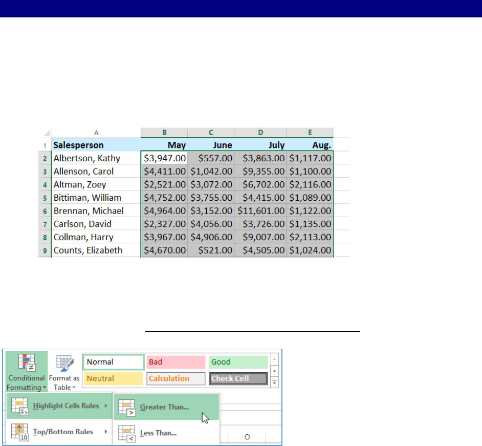
CONDITIONAL FORMATTING
Conditional Formatting is used to emphasize data that meets certain conditions in cells or
formulas. For example, you can set up Conditional Formatting so that all sales greater than or
equal to a value will display in a different color. The formatting options used for a condition can
be customized.
CREATE A CONDITIONAL FORMATTING RULE
In this example, a worksheet contains sales data and we'd like to see which salespeople are
meeting their monthly sales goals. The sales goal is $4,000 per month. Create a conditional
formatting rule for any cells containing a value higher than 4000.
1. Use the spreadsheet CONDFORMATTING in the workbook: AdvExcelExamples.xlsx
2. Select the desired cells for the conditional formatting rule. In this example, May, June,
July and August values were selected (do not select the column headings).
3. From the HOME tab, click the CONDITIONAL FORMATTING command.
4. Hover the mouse over the desired conditional formatting type and then select
the rule from the menu that appears. In this example, ‘Greater Than’ is selected
because you want to highlight cells that are greater than $4,000.
5. In the dialog box that appears, enter 4000 into the blank field. Then, select
a formatting style (Light Red Fill with Dark Red Text) from the drop-down menu. The
conditional formatting will be applied to the selected cells.
6. You can apply multiple conditional formatting rules to a cell range or worksheet, allowing
you to visualize different trends and patterns in your data. Select the same values (May,

4
June, July, August). Now Highlight cells that are less than $2,000. Choose ‘Less Than’, enter
2000 in the dialog box and select the formatting style Green Fill with Dark Green Text.
REMOVE CONDITIONAL FORMATTING
1. Click the CONDITIONAL FORMATTING command.
2. Hover the mouse over CLEAR RULES and choose which rules you wish to clear.
3. Click MANAGE RULES... to edit or delete individual rules. This is especially useful if you
have applied multiple rules to a worksheet. You must change the Show formatting rules
for: dropdown to This Worksheet to see all the rules on the spreadsheet.
CONDITIONAL FORMATTING PRESETS
Excel has a number of pre-defined styles, or presets, that you can use to quickly apply
conditional formatting to your data. They are grouped into three categories:
DATA BARS are horizontal bars added to each cell, much like a bar graph.
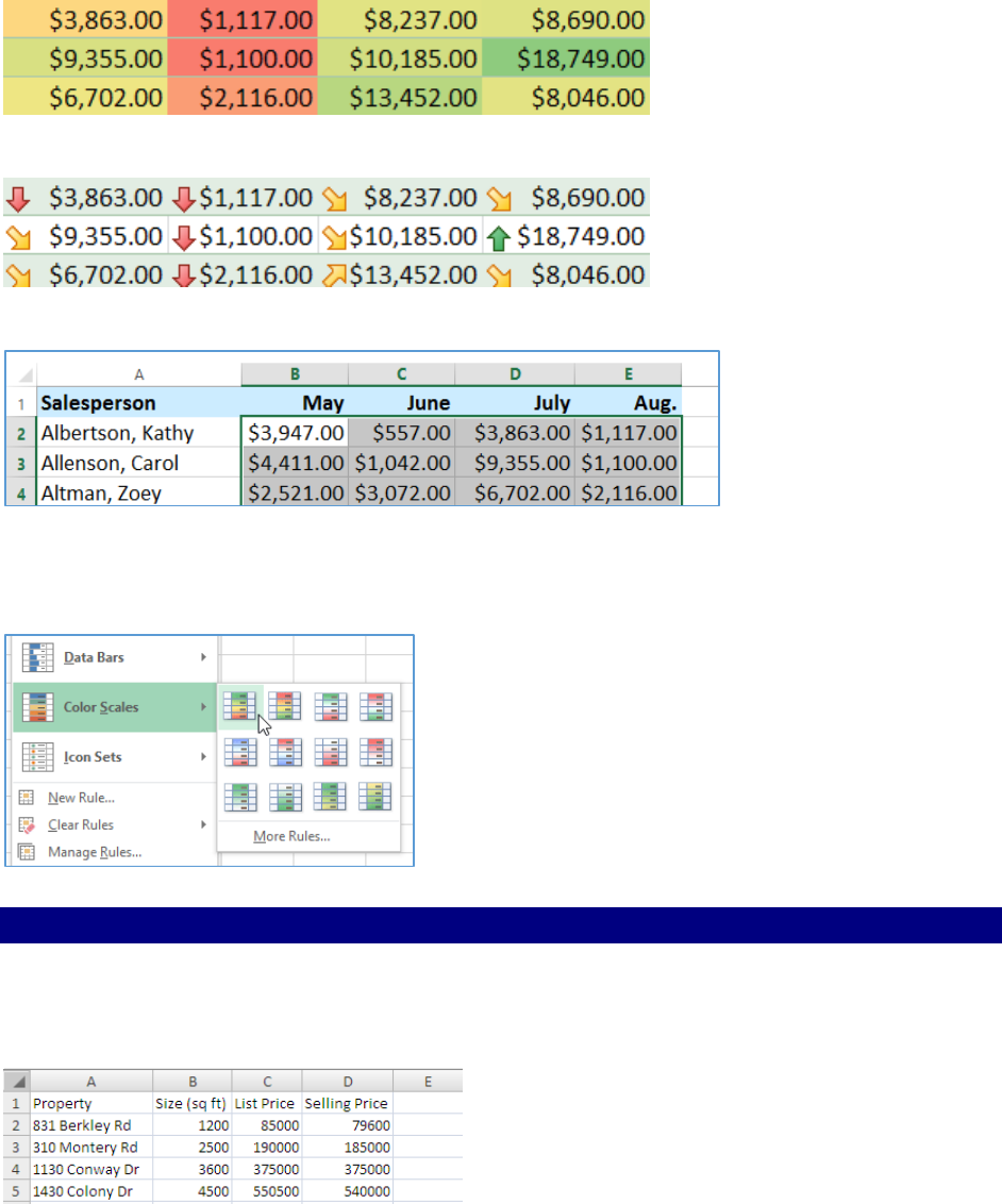
5
COLOR SCALES change the color of each cell based on its value. Each color scale uses
a two or three color gradient.
ICON SETS add a specific icon to each cell based on its value.
1. Select the desired cells for the conditional formatting rule.
2. Click the CONDITIONAL FORMATTING command.
3. Hover the mouse over the desired preset and then choose a preset style. The
conditional formatting will be applied to the selected cells.
HIGHLIGHT DUPLICATE ENTRIES
When you need to quickly compare two columns of data for duplicates entries, you can use
Excel’s conditional formatting with the COUNTIF function. For example, suppose you want to
know which properties’ selling prices matched their list prices in the worksheet shown below:
1. Select cells C2 thru D17.
2. Click CONDITIONAL FORMATTING and choose NEW RULE. Then, click Use A Formula To
Determine Which Cells To Format.
3. Enter the formula in the Format Values Where This Rule Is True text box and enter the
following formula:
= COUNTIF($C2:$D2,$C2)>1

6
4. Click the FORMAT button. On the FILL tab, select yellow under Background Color and
click OK. Click OK again to return to your worksheet.
USING STOP IF TRUE WHEN CONDITIONAL FORMATTING
When applying Conditional Formatting, you may have situations where you don’t want to
apply your rule to certain cells in a range.
1. In cell A21 type On, in cell A22 type Off and in cell B1 type Formatting: .
2. Select cells A21 and A22; name this range options.
3. Select cell C1 and click the DATA VALIDATION button from within the DATA tab.
4. Select DATA VALIDATION, choose LIST from the ALLOW dropdown and enter
=options as the SOURCE to populate the List box. Click OK.
Figure 7: Data Validation dialog box
Select the data range again and click the CONDITIONAL FORMATTING button. Choose
MANAGE RULES.
Click the NEW RULE button and choose Use a Formula to Determine Which Cells to
Format. Enter a formula similar to the one below – you are comparing the selection
from the list to the word “OFF”. If your selection = OFF, then don’t format; if it
doesn’t = OFF then apply formatting.
Remember to check STOP IF TRUE.

7
WORKING WITH CHARTS AND GRAPHS
ADDING SPARKLINES
SPARKLINES are miniature charts that you can put into a cell if you have a large table of figures.
Rather than making a chart that covers all the figures that sits somewhere else on the
worksheet, you can put a bar chart or a trend line into the last row or column of the table. That
way you can see exactly what’s happening in the numbers, all of which you can see at the same
time.
1. Open ADDSAL1.XLSX. Click on the QTR 1 tab to make it the active worksheet if it is not
currently active.
2. Select COLUMN E, click the right mouse button, and choose INSERT from the navigation
menu to add a new empty column to the right of column D.
3. Select cells B3 through D3 to use as the data for the sparkline.
4. From the SPARKLINE group on the INSERT tab, select the LINE sparkline.
5. Do one of the following to specify E3 as the target cell where you want the sparkline to
be placed:
Type E3 in the LOCATION RANGE box.
Click the Collapse Dialog button, , and select cell E3 with your mouse.

8
6. Click OK to insert the sparkline in cell E3.
7. To quickly add sparklines to cells E4 and E5, select cell E3 and use the Fill Handle in the
lower right corner of the cell to drag the sparkline format to cells E4 and E5.
8. To format the sparkline, click the DESIGN tab from the SPARKLINE TOOLS contextual tab
and choose from the preset options in the STYLE group.
CREATING A QUICK CHART
EXERCISE: CREATING A QUICK CHART
1. If using OIT Training Room files, open the file ADDSAL1.xlsx.
2. Click the QTR1 worksheet tab and select the 3 month data for the salespersons.
3. Press the [F11] key. A basic column chart will be created on a new tab.
4. With the new chart open, click the CHANGE CHART TYPE button in the TYPE group on
the DESIGN tab.
5. The Change Chart Type window will open. Select BAR in the Navigation Pane, and select
the first choice (if it is not already selected). Then, click OK.
6. To change the chart back, simply reselect the COLUMN style repeating the steps above.

9
CREATING A STANDARD CHART
5. Select the data in cells A2:D6.
6. Click the INSERT tab and click the COLUMN CHART button.
7. Select the CLUSTERED COLUMN choice under 2D CHARTS. The chart will be created in
the 1
st
Qtr worksheet.
8. To move the chart to a separate sheet, click the MOVE CHART LOCATION button, and
select NEW SHEET.
9. Name the chart “MY CHART”.
CHARTING NON-ADJACENT RANGES
You to chart Non-Adjacent Ranges, which are ranges of cells that are not located next to each
other.
1. Select the first range of cells that you want to chart.
2. Hold down the [CTRL] key and select the next range of cells.
3. Click on the INSERT tab, and select the appropriate chart type.
FORMATTING THE CHART
CHART STYLES
There are numerous Chart Styles available in the CHART STYLES group on the DESIGN tab. Click
the UP and DOWN arrows to view additional choices or click the MORE button to see all the
style options. Click on the style to apply it to your chart.
CHART LAYOUT
Basic Chart Layout options are available in the CHART LAYOUT group on the DESIGN tab. Note
that these layout options are visually displayed in the selection buttons.
Extensive Chart Layout options are available on the Layout tab. From this tab, you can
customize the Primary Horizontal and Vertical Axes, add a Trendline or Data Table, and add
additional text to your graph.
EXERCISE: CHANGING THE CHART LAYOUT
1. Click the first CHART LAYOUT button, . The layout will change.
2. Click on the CHART TITLE text box.
3. Select the text “CHART TITLE” and type in FIRST QUARTER.

10
FORMATTING THE AXIS
By default, charts will have a Primary Horizontal and Vertical axis. These axes can be formatted
or deleted entirely. The axes can be selected by clicking the AXES button and then selecting
either PRIMARY HORIZONTAL or PRIMARY VERTICAL AXIS and, then selecting a display choice.
For additional formatting, select MORE PRIMARY VERTICAL (OR HORIZONTAL) AXIS OPTIONS.
You may also right-click directly on the AXIS and select FORMAT AXIS from the menu.
1. From the MY CHART worksheet tab, click the LAYOUT tab.
2. Right-click on the VERTICAL axis and select FORMAT AXIS from the menu. The FORMAT
AXIS window will open.
3. Select NUMBER under AXIS OPTIONS. Select CURRENCY under Category, and change
the DECIMAL PLACES to 0.
4. Click CLOSE.
FORMATTING AXIS TITLES
By default, charts will not have Axis titles. You can create Axis titles by selecting the AXIS TITLES
button and selecting either PRIMARY HORIZONTAL or PRIMARY VERTICAL AXIS TITLES, and
then selecting a display choice. For additional formatting, select MORE PRIMARY VERTICAL (OR
HORIZONTAL) AXIS TITLES OPTIONS.
EXERCISE: FORMATTING THE AXES TITLES
1. Click the AXIS TITLES button and select PRIMARY HORIZONTAL AXIS TITLE.
2. Select TITLE BELOW AXIS.
3. Click in the AXIS TITLE text box and replace the text “AXIS TITLE” with SALESPERSON.
4. Next, click the AXIS TITLES button and select PRIMARY VERTICAL AXIS TITLE.
5. Click in the AXIS TITLE text box and replace the text “AXIS TITLE” with MONTHLY SALES.

11
FORMATTING GRIDLINES
By default, charts created in Excel 2016 will have Primary Horizontal gridlines for major chart
tracking units. These gridlines can be formatted or deleted entirely. Also, Vertical gridlines can
be added to the chart. Gridlines can be selected by clicking the GRIDLINES button and
selecting either PRIMARY HORIZONTAL or PRIMARY VERTICAL GRIDLINES, and then selecting a
display choice. For additional formatting, select MORE PRIMARY VERTICAL (OR HORIZONTAL)
GRIDLINES OPTIONS.
You may also right-click directly on a GRIDLINE and select FORMAT GRIDLINES from the menu.
ADDING A DATA TABLE
A Data Table is a table that displays all the ranges and labels that were used to create a chart.
Data tables are useful when you want to explain the details of a chart during a presentation, or
when exact figures need to be shown. Data tables are placed below the chart and can include a
legend key.
1. Click the DATA TABLE button.
2. Select SHOW DATA TABLE.
ADDING DATA LABELS
Data Labels display the exact values of the data in a chart next to the graphic objects they
represent. These values help add clarity to the chart. Data labels can be added to any chart
type, but they are usually used for pie charts, due to space limitations.
To add a Data Label to a chart, click the DATA LABELS button . Then, select a placement choice.
For additional formatting, select MORE DATA LABEL OPTIONS.
12
ADDING A TRENDLINE
Because of the varying height of the bars in a column chart, it is sometimes difficult to
determine the general direction of the action. Excel enables you to quickly add a Trendline to a
data series. A trendline has the effect of smoothing out the rough spots in a chart and gives you
a better picture of the data series.
To add a Trendline to a chart, click the TRENDLINE button. Then select a trendline style. The
ADD TRENDLINE window will open. Select the SERIES you wish to base the trendline on and
click OK. You can also click on the data series directly in the chart.
EXERCISE: ADDING A TRENDLINE
1. Click the TRENDLINE button. The ADD TRENDLINE window will open.
2. Select JAN and click OK.
3. To remove the trendline, click the TRENDLINE BUTTON. Then select NONE.
APPLYING CHART THEMES
In addition to the built-in Chart Styles featured on the DESIGN tab, there are a number of built
in Themes, located on the PAGE LAYOUT tab, that can be applied to instantly format your chart.
CHANGING COLORS OF INDIVIDUAL DATA SERIES
You can choose to customize the color or style of an individual Data Series to highlight the
series within a chart by selecting and formatting the series.
1. Click the March data series. Then, select Format Data Series.
o After selecting a series, click once on a single item in the series to select just
that one data series.
2. Select Fill under series options.
3. Select Solid Fill.
4. Click the color button, ,and select red from the color-picker.

13
INSERTING GRAPHICS ELEMENTS IN YOUR DATA SERIES
1. Create a bar or column chart and select one of the data series.
2. Right click and select Format Data Series.
3. Select fill, picture or texture fill.
4. Select file or online and, then, select an image.
5. Select stack.
(snow in january, february, and
march; rain in april and may.)
CREATING A COMBINATION CHART
Change one of the axis in a bar chart to a line chart
1. Select the data series that you want to change.
2. Right click and select change series chart type.
3. Select line and choose a line chart type.
4. press ok, and the line appears over the top of the other series bar.

14
PIE OF PIE CHART
To make smaller slices more visible in a pie chart, Excel provides the PIE OF PIE and BAR OF PIE
chart sub-types.
1. Create the data that you want to use as follows:
2. Select the data range, in this example, highlight cell A2:B9. Click Insert > Pie > Pie of
Pie or Bar of Pie:
3. And you will get the following chart:
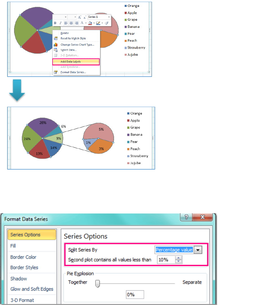
15
4. You can add the data labels for the data points of the chart; select the pie chart and
right click, choose Add Data Labels:
5. Right-click and choose Format Data Series from the context menu
6. In the Format Data Series dialog, click the drop down list beside Split Series By to
select Percentage value, then set the value you want to display in the second pie, in this
example, choose 10% .

16
7. Close the dialog box:
If you created the Bar of pie chart, you will get the following:
ADD BACKGROUND PICTURE
If you want to add a picture or your company’s logo as background to the chart:
1. Select your chart and right click, then choose Format Chart Area.
2. Check Picture or texture fill radio button under Fill option, click File or Clipboard or Clip
Art button under Insert from section to select a picture or clip art, change the
transparency.

17
GROUPS AND SUBTOTALS
Worksheets with a lot of content can sometimes feel overwhelming and even become difficult
to read. Fortunately, Excel can organize data in groups, allowing you to easily show and hide
different sections of your worksheet. You can also summarize different groups using the
Subtotal command and create an outline for your worksheet.
TO GROUP ROWS OR COLUMNS:
1. Select the rows or columns you want to group. In this example, we'll select columns A,
B, and C.
2. Select the Data tab on the Ribbon, then click the Group command.
3. The selected rows or columns will be grouped.
To ungroup data, select the grouped rows or columns, then click the Ungroup command.
TO HIDE AND SHOW GROUPS:
1. To hide a group, click the Hide Detail button .
2. The group will be hidden. To show a hidden group, click the Show Detail button .
18
CREATING SUBTOTALS
The Subtotal command allows you to automatically create groups and use common functions
like SUM, COUNT, and AVERAGE to help summarize your data. For example, the Subtotal
command could help to calculate the cost of office supplies by type from a large inventory
order. It will create a hierarchy of groups, known as an outline, to help organize your
worksheet.
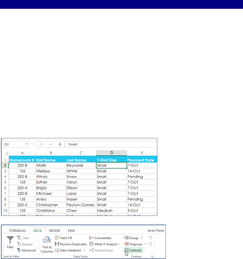
Your data must be correctly sorted before using the Subtotal command.
We will use the Subtotal command with a T-shirt order form to determine how many T-shirts
were ordered in each size (Small, Medium, Large, and X-Large). This will create an outline for
our worksheet with a group for each T-shirt size and then count the total number of shirts in
each group.
1. First, sort your worksheet by the data you want to subtotal. In this example, we will
create a subtotal for each T-shirt size, so our worksheet has been sorted by T-shirt size
from smallest to largest.
2. Select the Data tab, then click the Subtotal command.
3. The Subtotal dialog box will appear. Click the drop-down arrow for the At each change
in: field to select the column you want to subtotal. In our example, we'll select T-Shirt
Size.
4. Click the drop-down arrow for the Use function: field to select the function you want to
use. In our example, we'll select COUNT to count the number of shirts ordered in each
size.
5. In the Add subtotal to: field, select the column where you want the calculated subtotal
to appear. In our example, we'll select T-Shirt Size.

19
6. When you're satisfied with your selections, click OK.
7. The worksheet will be outlined into groups, and the subtotal will be listed below each
group. In our example, the data is now grouped by T-shirt size, and the number of shirts
ordered in that size appears below each group.
TO VIEW GROUPS BY LEVEL
When you create subtotals, your worksheet it is divided into different levels. You can switch
between these levels to quickly control how much information is displayed in the worksheet by
clicking the Level buttons image of button for levels 1, 2, 3 to the left of the worksheet.
1. Click the lowest level to display the least detail. In our example, we'll select level 1,
which contains only the grand count, or total number of T-shirts ordered.
2. Click the next level to expand the detail. In our example, we'll select level 2, which
contains each subtotal row but hides all other data from the worksheet.
3. Click the highest level to view and expand all of your worksheet data.
TO REMOVE SUBTOTALS
Sometimes you may not want to keep subtotals in your worksheet, especially if you want to
reorganize data in different ways. If you no longer want to use subtotaling, you'll need remove
it from your worksheet.
1. Select the Data tab, then click the Subtotal command.
2. The Subtotal dialog box will appear. Click Remove All.

20
TABLES
Just like regular formatting, tables can improve the look and feel of your workbook, and they'll
also help you organize your content and make your data easier to use. Excel includes several
tools and predefined table styles, allowing you to create tables quickly and easily.
INSERT A TABLE
1. Click any single cell inside the data set.
2. On the INSERT tab, click TABLE.
3. Excel automatically selects the data. Check 'My table has headers' and click OK.
This may still seem like a normal data range to you but many powerful features are now just a
click of a button away. The TABLE TOOLS contextual tab (with the underlying Design tab
selected) is the starting point for working with tables. If at any time you lose this tab, simply
click any cell within the table and it will activate again.

21
SORT A TABLE
To sort by Last Name first and Sales second, first sort by Sales, next sort by Last Name (the
exact opposite).
1. Click the arrow next to Sales and click Sort Smallest to Largest.
2. Click the arrow next to Last Name and click Sort A to Z.
FILTER A TABLE
1. Click the arrow next to Country and only check USA.

22
Filters are cumulative, which means you can apply multiple filters to help narrow down your
results.
2. Click the drop-down arrow for the column you want to filter.
3. The Filter menu will appear.
4. Check or uncheck the boxes depending on the data you want to filter, then click OK.
5. The new filter will be applied.
ADVANCED FILTERS
If the data you want to filter requires complex criteria (such as Type = "Produce" OR
Salesperson = "Davolio") you can use the Advanced Filter dialog box.
The Advanced command works differently from the Filter command in several important ways.
It displays the Advanced Filter dialog box instead of the AutoFilter menu.
You type the advanced criteria in a separate criteria range on the worksheet and above
the range of cells or table you want to filter.
o Excel uses the separate criteria range in the Advanced Filter dialog box as the
source for the advanced criteria.
23
WILDCARD CRITERIA
Boolean logic: Salesperson = a name with 'u' as the second letter
To find text values that share some characters but not others, do one or more of the following:
Type one or more characters without an equal sign (=) to find rows with a text value in a
column that begin with those characters. For example, if you type the text Dav as a
criterion, Excel finds "Davolio," "David," and "Davis."
Use a wildcard character.
Use
To find
? (question mark)
Any single character
For example, sm?th finds "smith" and "smyth"
* (asterisk)
Any number of characters
For example, *east finds "Northeast" and "Southeast"
~ (tilde) followed by ?, *, or ~
A question mark, asterisk, or tilde
For example, fy91~? finds "fy91?"
24
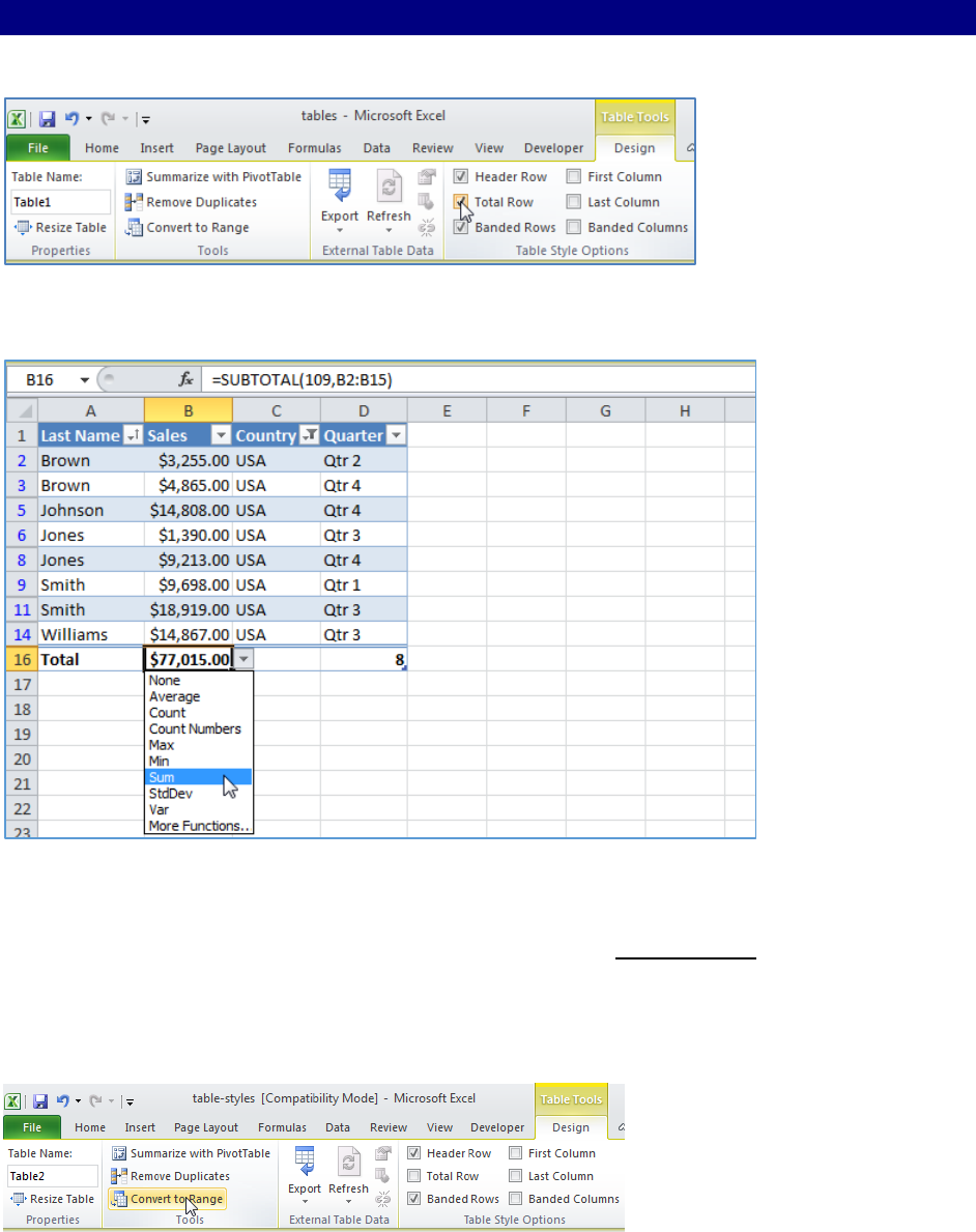
TOTAL ROW
1. On the DESIGN tab, in the TABLE STYLE OPTIONS group, check Total Row.
2. Click any cell in the last row to calculate the TOTAL of a column. For example, calculate
the sum of the Sales column.
Note: in the formula bar see how Excel uses the SUBTOTAL function to calculate the sum. 109 is
the argument for Sum if you use the SUBTOTAL function. Excel uses this function (and not the
standard SUM function) to correctly calculate table totals of filtered tables.
To convert this table back to a normal range of cells (and keep the formatting), execute the
following steps.
3. On the DESIGN tab, in the TOOLS group, click CONVERT TO RANGE.
Note: to remove the table style, select the range of cells, on the HOME tab, in the STYLES
group, click NORMAL.

25
PIVOT TABLES
A pivot table allows you to extract the significance from a large, detailed data set.
To insert a pivot table:
1. Click any single cell inside the data set.
2. On the Insert tab, click PivotTable.
The following dialog box appears. Excel automatically selects the data for you. The default
location for a new pivot table is New Worksheet.
3. Click OK.

26
Once you create a PivotTable, you'll need to decide which fields to add. Each field is simply a
column header from the source data. In the PivotTable Field List, check the box for each field
you want to add.
In our example, we want to know the total amount sold by each salesperson, so we'll check the
Salesperson and Order Amount fields.
The selected fields will be added to one of the four areas below. In our example, the
Salesperson field has been added to the Rows area, while Order Amount has been added to
Values. Alternatively, you can drag and drop fields directly into the desired area.
The PivotTable will calculate and summarize the selected fields. In our example, the PivotTable
shows the amount sold by each salesperson.

27
Pivoting data
One of the best things about PivotTables is that they can quickly pivot—or reorganize—your
data, allowing you to examine your worksheet in several ways. Pivoting data can help you
answer different questions and even experiment with your data to discover new trends and
patterns.
To add columns:
So far, our PivotTable has only shown one column of data at a time. In order to show multiple
columns, you'll need to add a field to the Columns area.
Drag a field from the Field List into the Columns area. In our example, we'll use the Month
field.
The PivotTable will include multiple columns. In our example, there is now a column for each
person's monthly sales, in addition to the Grand Total.
28
To change a row or column:
Changing a row or column can give you a completely different perspective on your data. All you
have to do is remove the field in question, then replace it with another.
Drag the field you want to remove out of its current area. You can also uncheck the appropriate
box in the Field List. In this example, we've removed the Month and Salesperson fields.
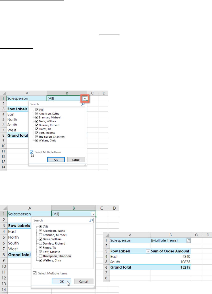
To add a filter:
In the example below, we'll filter out certain salespeople to determine how their individual
sales are impacting each region.
The filter will appear above the PivotTable. Click the drop-down arrow, then check the box next
to Select Multiple Items.
Uncheck the box next to any item you don't want to include in the PivotTable. In our example,
we'll uncheck the boxes for a few salespeople, then click OK. The PivotTable will adjust to
reflect the changes.

29
Slicers
Slicers make filtering data in PivotTables even easier. Slicers are basically just filters but are
easier and faster to use, allowing you to instantly pivot your data. If you frequently filter your
PivotTables, you may want to consider using slicers instead of filters.
To add a slicer:
Select any cell in the PivotTable.
From the Analyze tab, click the Insert Slicer command.
A dialog box will appear. Check the box next to the desired field. In our example, we'll
select Salesperson, then click OK.
The slicer will appear next to the PivotTable. Each selected item will be highlighted in blue. In
the example below, the slicer contains all eight salespeople, but only five of them are currently
selected.
Just like filters, only selected items are used in the PivotTable. When you select or deselect an
item, the PivotTable will instantly reflect the change. Press and hold the Ctrl key on your
keyboard to select multiple items at once.

30
PIVOT CHART
A pivot chart is the visual representation of a pivot table in Excel. Pivot charts and pivot tables
are connected with each other.
By design, a Pivot Chart never displays data from the Grand Total column of a Pivot Table. The
Select Data button on the Pivot Chart Tools/Design tab does not allow the user to reselect the
Source data to include the Grand Total column. The only option left in this case is to copy the
Pivot Table and paste it as Paste Special > Values in another range and then create a chart from
this data. But in doing so, any change in the slicer or Base data will not have any effect on the
Chart because the source of the Chart is a static range.

31
Column F – enter 1/1/2008, use Fill Handle for date (difference b/w left & right mouse
button)
Column G - =TEXT(DATE(YEAR(F2),MONTH(F2),DAY(F2)),"mmmm")
Column H – calculate which Quarter of the year is the month, then add a ‘Q’ in front of
it (we won’t be using the Quarter as a number, so this is just extra formatting for a nicer
display (optional))
=”Q” & INT((MONTH(F2)+2)/3) &”-“& YEAR(A2)
Column I - =YEAR(F2)
If adding additional years (2011, 2012, etc), and you need Revenue data, use the
RANDBETWEEN(bottom,top) function. Remember to copy/paste as value to remove the
formula.

32

33
Using GETPIVOT() to Link Values
To have the copy/paste data (from above example) automatically refresh, link the Grand Total
values between the two tables. Type an equal sign, =, in the cell, and, then, click the Grand
Total cell in the Pivot Table to create a linked formula.
