Complete ABAP

Reading Sample

In this reading sample, we provide two sample chapters. The first

sample chapter introduces basic ABAP programming language con-

cepts, which lay the foundation to writing ABAP programs. The

second sample chapter discusses how to implement object-oriented

programming techniques such as encapsulation, inheritance, and

polymorphism in your code.

Kiran Bandari

Complete ABAP

1047 Pages, 2016, $79.95

ISBN 978-1-4932-1272-9

www.sap-press.com/3921

First-hand knowledge.

“ABAP Programming Concepts”

“Object-Oriented ABAP”

Contents

Index

The Author

107

Chapter 4

In this chapter, we’ll look at basic ABAP programming language concepts.

The concepts discussed in this chapter will lay the foundations to write

your own ABAP programs.

4 ABAP Programming Concepts

ABAP programs process data from the database or an external source. As discussed

in Chapter 2, ABAP programs run in the application layer, and ABAP program

statements can work only with locally available data in the program. External data,

like user inputs on screens, data from a sequential file, or data from a database ta-

ble, must always be transported to and saved in the program’s local memory in or-

der to be processed with ABAP statements.

In other words, before any data can be processed with an ABAP program, it must

first be read from the source, stored locally in the program memory, and then

accessed via ABAP statements; you can’t work with the external data directly

using ABAP statements. This temporary data that exists in an ABAP program

while the program is executed is called transient data and is cleared from memory

once the program execution ends. If you wish to access this data later, it must be

stored persistently in the database; such stored data is called persistent data.

This chapter provides information on the basic building blocks of the ABAP pro-

gramming language in order to understand the different ways to store and pro-

cess data locally in ABAP programs. In Section 4.1, we begin by looking at the

general structure of an ABAP program, before diving into ABAP syntax rules and

ABAP keywords in Section 4.2 and Section 4.3, respectively.

Section 4.4 introduces the

TYPE concept, and explores key elements such as data

types and data objects, which define memory locations in ABAP programs to

store data locally. In Section 4.5, we discuss the different types of ABAP state-

ments that can be employed, including declarative, modularization, control, call,

and operational statements. Finally, in Section 4.6, we conclude this chapter by

walking through the steps to create your first ABAP program!

ABAP Programming Concepts

108

Initially, we’ll use a procedural model for our examples to keep things simple;

we’ll switch to an object-oriented model after we discuss object-oriented pro-

gramming in Chapter 8.

4.1 General Program Structure

Any ABAP program can be broadly divided into two parts:

왘

Global declarations

In the global declaration area, global data for the program is defined; this data

can then be accessed from anywhere in the program.

왘

Procedural

The procedural part of the program consists of various processing blocks such

as dialog modules, event blocks, and procedures. The statements within these

processing blocks can access the global data defined in the global declarations.

In this section, we’ll look at both of these program structure parts.

4.1.1 Global Declarations

The global declaration part of an ABAP program uses declarative statements to

define memory locations, which are called data objects and which store the work

data of the program. ABAP statements work only with data available in the pro-

gram as content for data objects, so it’s imperative that data is stored in a data

object before it’s processed by an ABAP program.

Data objects are local to the program; they can be accessed via ABAP statements

in the same program. The global declaration area exists at the top of the program

(see Figure 4.1). We use the term global with respect to the program; data objects

defined in this area are visible and valid throughout the entire ABAP program and

can be accessed from anywhere in the source code using ABAP statements.

ABAP also uses local declarations, which can be accessed only within a subset of

the program. We’ll explore local declarations in Chapter 7 when we discuss mod-

ularization techniques.

General Program Structure

4.1

109

Figure 4.1 Program Structure

4.1.2 Procedural

After the declarative area is the procedural portion of the program. Here, the pro-

cessing logic of the ABAP program is defined. In this section of the ABAP pro-

gram, you typically use various ABAP statements to import and process data from

an external source.

The procedural area is where the program logic is implemented. It uses various

processing blocks that contain ABAP statements to implement business require-

ments. For example, in a typical report, the procedural area contains an event

block to process the selection screen and validate user inputs on the selection

screen and another event block to fetch the data from the database based on user

input, and then calls a procedure to display the output to the user.

Declaration Part

Procedural Part

ABAP Programming Concepts

110

4.2 ABAP Syntax

The source code of an ABAP program is simply a collection of various ABAP state-

ments, interpreted by the runtime environment to perform specific tasks. You use

declarative statements to define data objects, modularization statements to define

processing blocks, and database statements to work with the data in the database.

In this section, we’ll look at the basic syntax rules that every ABAP programmer

should know. We’ll then look at the use of chained statements and comment

lines.

4.2.1 Basic Syntax Rules

There are certain basic syntax rules that need to be followed while writing ABAP

statements:

왘 An ABAP program is a collection of individual ABAP statements that exist

within the program. Each ABAP statement is concluded with a period (".") and

the first work of the statement is known as a keyword.

왘 An ABAP statement consists of operands, operators, or additions to keywords

(see Figure 4.2). The first word of an ABAP statement is an ABAP keyword, the

remaining can be operands, operators, or additions. Operands are the data

objects, data types, procedures, and so on.

Various operators are available, such as assignment operators that associate the

source and target fields of an assignment (e.g.,

= or ?=), arithmetic operators

that assign two or more numeric operands with an arithmetic expression (e.g.,

+, -, *), relational operators that associate two operands with a logical expres-

sion (such as

=, <, >), etc. Each ABAP keyword will have its own set of additions.

왘 Each word in the statement must be separated by at least one space.

왘 An ABAP statement ends with a period, and you can write a new statement on

the same line or on a new line. A single ABAP statement can extended over sev-

eral lines.

왘 ABAP code is not case-sensitive.

In Figure 4.2, the program shown consists of three ABAP statements written

across three lines. The first word in each of these statements (

REPORT, PARAMETERS,

ABAP Syntax

4.2

111

and WRITE) is a keyword. As you can see, each statement begins with a keyword

and ends with a period. Also, each ABAP word is separated by a space.

Figure 4.2 ABAP Statement

You can write multiple statements on one line or one statement can extend over

multiple lines. Therefore, if you wish, you can rewrite the code in Figure 4.2 as

shown:

REPORT ZCA_DEMO_PROGRAM. PARAMETERS p_input(10) TYPE c. WRITE p_

input RIGHT-JUSTIFIED.

However, to keep the code legible, we recommend restricting your program to

one statement per line. In some cases, it’s recommended to break a single state-

ment across multiple lines—for example:

SELECT * FROM mara INTO TABLE it_mara WHERE matnr EQ p_matnr.

The above statement may be written as shown in Listing 4.1 to make it more leg-

ible.

SELECT * FROM mara

INTO TABLE it_mara

WHERE matnr EQ p_matnr.

Listing 4.1 Example of Splitting Statement across Multiple Lines

4.2.2 Chained Statements

If more than one statement starts with the same keyword, you can use a colon (:)

as a chain operator and separate each statement with a comma. These are called

chained statements, and they help you avoid repeating the same keyword on each

line.

For example,

DATA v_name(20) TYPE c.

DATA v_age TYPE i.

Keyword Operand Addition

ABAP Programming Concepts

112

Also can be written as

DATA : v_name(20) TYPE c,

v_age TYPE i.

End the last statement in the chain with a period. Chained statements are not lim-

ited to keywords; you can put any identical first part of a chain of statements

before the colon and write the remaining parts of the individual statements sepa-

rated by comma—for example,

v_total = v_total + 1.

v_total = v_total + 2.

v_total = v_total + 3.

v_total = v_total + 4.

can be chained as

v_total = v_total + : 1, 2, 3, 4.

Note

ABAP code is not case-sensitive, so you can use either uppercase or lowercase to write

ABAP statements. We recommend writing keywords and their additions in uppercase

and using lowercase for other words in the statement to make the code more legible.

4.2.3 Comment Lines

To make your source code easy to understand for other programmers, you can

add comments to it (see Listing 4.2). Comment lines are ignored by the system

when the program is generated, and they’re useful in many ways.

DATA f1 TYPE c LENGTH 2 VALUE 'T3'.

DATA f2 TYPE n LENGTH 2.

*This is a comment line

f2 = f1.

WRITE f2. "This is also a comment line

Listing 4.2 Comment lines

There are two ways to add comment lines in source code:

왘 You can enter an asterisk (

*) at the beginning of a line to make the entire line

a comment.

왘 You can enter a double quotation mark (

") midline to make the part of the line

after the quotation mark a comment this is called an in-line comment).

ABAP Keywords

4.3

113

You can comment (i.e., set as a comment) on a block of lines at once (a multiline

comment) by selecting the lines to be commented on and pressing

(Ctrl) + (<) on

the keyboard. Similarly, to uncomment (i.e., set as normal code) a block of lines,

you can select the lines and press (Ctrl) + (>).

Alternatively, you can also use the context menu to comment or uncomment

code. To comment a line of code or a block lines, select the code, right-click, and

select the appropriate option from the Format context menu. This helps you

avoid the tedious job of adding asterisks manually at the beginning of each line.

Now that you have a better understanding of basic ABAP syntax rules and chain-

ing ABAP statements, in the next section, we’ll look at the keywords used in

ABAP.

4.3 ABAP Keywords

Because each ABAP statement starts with a keyword, writing ABAP statements is

all about choosing the right keyword to perform the required task. Every key-

word provides specific functionality and comes with its own set of additions,

which allow you to extend the keyword’s functionality.

For each keyword, SAP maintains extensive documentation, which serves as a

guide to understanding the syntax to use with the keyword and the set of addi-

tions supported for the keyword.

You can access the keyword documentation by typing “ABAPDOCU” in the com-

mand bar to open it just like any other transaction or by placing the cursor on the

keyword and pressing

(F1) while writing your code in ABAP Editor. You can also

visit https://help.sap.com/abapdocu_750/en/abenabap.htm, to access an online ver-

sion of the ABAP keyword documentation (see Figure 4.3).

Because there are literally hundreds of keywords that can be used in ABAP, the

best way to become familiar with the keywords is to explore them in relation to

a requirement. We’ll be taking this approach throughout the book as we intro-

duce you to these keywords in various examples.

ABAP Programming Concepts

114

Figure 4.3 ABAP Keyword Documentation

4.4 Introduction to the TYPE Concept

An ABAP program only works with data inside data objects. The first thing you

do when developing a program is declare data objects. Inside these data objects,

you store the data to be processed in your ABAP program. You use declarative

statements to define data objects that store data in the program; these statements

are called data declarations.

Typically, you’ll work with various kinds of data, such as a customer’s name,

phone number, or amount payable. Each type of data has specific characteristics.

The customer’s name consists of letters, a phone number consists of digits from 0

to 9, and the amount due to the customer will be a number with decimal values.

Identifying the type and length of data that you plan to store in data objects is

what the

TYPE concept is all about.

In this section, we’ll look at data types, domains, and data objects.

Introduction to the TYPE Concept

4.4

115

4.4.1 Data Types

Data types are templates that define data objects. A data type determines how the

contents of a data object are interpreted by ABAP statements. Other than occupy-

ing some space to store administrative information, they don’t occupy any mem-

ory space for work data in the program. Their purpose simply is to supply the

technical attributes of a data object.

Data types can be broadly classified as elementary, complex, or reference types.

In this chapter, we’ll primarily explore the elementary data types and will only

briefly cover complex types and reference types. More information on complex

data types can be found in Chapter 5, and more details about reference types are

provided in Chapter 8.

Elementary Data Types

Elementary data types specify the types of individual fields in an ABAP program.

Elementary data types can be classified as predefined elementary types or user-

defined elementary types. We’ll look at these subtypes next.

Predefined Elementary Data Types

The SAP system comes built in with predefined elementary data types. These data

types are predefined in the SAP NetWeaver AS ABAP kernel and are visible in all

ABAP programs. You can use these predefined elementary data types to assign a

type to your program data objects. You can also create your own data types (user-

defined elementary data types) by referring to the predefined data types.

Table 4.1 lists the available predefined elementary data types.

Data Type Definition

i Four-byte integer

int8 Eight-byte integer

f Binary floating-point number

p Packed number

decfloat16 Decimal floating-point number with sixteen decimal places

decfloat34 Decimal floating-point number with thirty-four decimal places

Table 4.1 Predefined Elementary Data Types

ABAP Programming Concepts

116

Predefined elementary data types can be classified as numeric or nonnumeric

types. There are six predefined numeric elementary data types:

왘 4-byte integer (

왘 8-byte integer (

int8)

왘 Binary floating-point number (

왘 Packed number (

왘 Decimal floating point number with 16 decimal places (

decfloat16)

왘 Decimal floating point number with 34 decimal places (

decfloat34)

There are five predefined nonnumeric elementary data types:

왘 Text field (

왘 Numeric character string (

왘 Date (

왘 Time (

왘 Hexadecimal (

The field length for data types

f, i, int8, decfloat16, decfloat34, d, and t is

fixed. In other words, you don’t need to specify the length when you use these

data types to declare data objects (or user-defined elementary data types) in your

program. The field length determines the number of bytes that the data object

occupies in memory. In types

c, n, x, and p, the length is not part of the type defi-

nition. Instead, you define it when you declare the data object in your program.

c Text field

(alphanumeric characters)

d Date field

(format: YYYYMMDD)

n Numeric text field

(numeric characters 0 to 9)

t Time field

(format: HHMMSS)

x Hexadecimal field

Data Type Definition

Table 4.1 Predefined Elementary Data Types (Cont.)

Introduction to the TYPE Concept

4.4

117

Before we discuss the predefined elementary data types further, let’s see how

they’re used to define a data object in the program.

The keyword used to define a data object is

DATA. For the syntax, you provide a

name for your data object and use the addition

TYPE to refer it to a data type, from

which the data object can derive its technical attributes.

For example, the line of code in Figure 4.4 defines the data object

V_NAME of TYPE

(character).

Figure 4.4 Declaring a Data Object

Notice that we did not specify the length in Figure 4.4; therefore, the object will

take the data type’s initial length by default. Here,

V_NAME will be a data object of

TYPE c (text field) and LENGTH 1 (default length). It can store only one alphanu-

meric character.

If you wish to have a different length for your data object, you need to specify the

length while declaring the data object, either with parentheses or using the addi-

tion

LENGTH:

DATA v_name(10) TYPE c.

DATA v_name TYPE c LENGTH 10.

In this example, V_NAME will be a data object of TYPE c and LENGTH 10. It can now

store up to 10 alphanumeric characters. The Valid Field Length column in Table

4.2 lists the maximum length that can be assigned to each data type.

For data types of fixed lengths, you don’t need to specify the length, because it’s

part of the

TYPE definition—for example:

DATA count TYPE i.

DATA date TYPE d.

Table 4.2 lists the initial length of each data type, its valid length, and its initial

value. The initial length is the default length that the data object occupies in mem-

ory if no length specification is provided while defining the data object, and the

initial value of a data object is the value it stores when the memory is empty.

Keyword Data Object Name Data Type Reference

ABAP Programming Concepts

118

For example, as shown in Table 4.2, a TYPE c data object will be filled with spaces

initially, whereas a

TYPE n data object would be filled with zeros.

Predefined nonnumeric data types can be further classified as follows:

왘

Character types

Data types c, n, d, and t are character types. Data objects of these types are

known as character fields. Each position in one of these fields can store one

code character. For example, a data object of

LENGTH 5 can store five characters

and a data object of

LENGTH 10 can store ten characters. Currently, ABAP only

works with single-byte codes, such as American Standard Code for Information

Interchange (ASCII) and Extended Binary Coded Decimal Interchange Code

(EBCDI). As of release 6.10, SAP NetWeaver AS ABAP supports both Unicode

and non-Unicode systems. However, support for non-Unicode systems has

been withdrawn from SAP NetWeaver 7.5.

Data Type Initial Field Length

(Bytes)

Valid Field Length

(Bytes)

Initial Value

Numeric Types

i 4 4 0

int8 8 8 0

f 8 8 0

p 8 1–16 0

decfloat16 8 8 0

decfloat34 16 16 0

Character Types

c 1 1–65535 Space

d 8 8 '00000000'

n 1 1–65535 '0 … 0'

t 6 6 '000000'

Hexadecimal Type

x 1 1–65535 X'0 … 0'

Table 4.2 Elementary Data Types: Technical Specifications

Introduction to the TYPE Concept

4.4

119

Single-byte code refers to character encodings that use exactly one byte for each

character. For example, the letter A will occupy one byte in single-byte encod-

ing.

ASCII is a character-encoding standard. ASCII code represents text in comput-

ers and other devices and is a popular choice for many modern character-

encoding schemes. In an ASCII file, each alphabetic or numeric character is rep-

resented with a seven-bit binary number.

EBCDI is an eight-bit character encoding, which means each alphabetic or

numeric character is represented with an eight-bit binary number.

왘

Hexadecimal types

The data type x interprets individual bytes in memory. These fields are called

hexadecimal fields. You can process single bits using hexadecimal fields. Hexa-

decimal notation is a human-friendly representation of binary-coded values.

Each hexadecimal digit represents four binary digits (bits), so a byte (eight bits)

can be more easily represented by a two-digit hexadecimal value.

With modern programming languages, we seldom need to work with data at the

bits and bytes levels. However, unlike ABAP (which uses single-byte code pages,

like ASCII), many external data sources use multibyte encodings. Therefore,

TYPE

fields are more useful in a Unicode system, in which you can work with the

binary data to be processed by an external software application.

For example, you can insert the hexadecimal code 09 between fields to create a

tab-delimited file so that spreadsheet software—like Microsoft Excel—knows

where each new field starts.

TYPE x fields are also useful if you wish to create files

in various formats from your internal table data.

Predefined Elementary ABAP Types with Variable Length

The data types we’ve discussed so far either have a fixed length or require a

length specification as part of data object declaration. We assume that we know

the length of the data we plan to process; for example, a material number is

defined in SAP as an alphanumeric field with a maximum of eighteen characters

in length. Therefore, if you wish to process a material number in your ABAP pro-

gram, you can safely create a data object as a

TYPE c field with LENGTH 18. How-

ever, there can be situations in which you need a field with dynamic length

because you won’t know the length of the data until runtime.

ABAP Programming Concepts

120

For such situations, ABAP provides data types with variable lengths:

왘

string

This is a character type with a variable length. It can contain any number of

alphanumeric characters.

왘

xstring

This is a hexadecimal type with a variable length.

When you define a

string as a data object, only the string header, which holds

administrative information, is created statically. The initial length of the

string

data object is 0, and its length changes dynamically at runtime based on the data

stored in the data object—for example:

DATA path TYPE string.

DATA xpath TYPE xstring.

Table 4.3 highlights some of the use cases for the predefined elementary data

types.

Data Type Use Case

Numeric Types

i Use to process integers like counters, indexes, time peri-

ods, and so on. Valid value range is -2147483648 to

+2147483647.

If the value range of

i is too small for your need, use

TYPE p without the DECIMALS addition.

Example syntax:

DATA f1 TYPE i. "fixed length

f Use to process large values when rounding errors aren’t

critical. To a great extent,

TYPE f is replaced by dec-

float

(decfloat16 and decfloat34) as of SAP Net-

Weaver AS ABAP 7.1.

Use data type

f only if performance-critical algorithms

are involved and accuracy is not important.

Example syntax:

DATA f1 TYPE f. "fixed length

Table 4.3 Predefined Elementary Data Types and Use Cases

Introduction to the TYPE Concept

4.4

121

p Use type p when fractions are expected with fixed deci-

mals known at design time (distances, amount of money

or quantities, etc.).

Example syntax:

DATA f1 TYPE p DECIMALS 2. "Takes default le

ngth 8

* OR you can manually specify length.

DATA f1(4) TYPE p DECIMALS 3.

decfloat16 and decfloat34 If you need fractions with a variable number of decimal

places or a larger value range, use

decfloat16 or dec-

float34

Example syntax:

DATA f1 TYPE decfloat16.

DATA f1 TYPE decfloat34.

Nonnumeric Types

c Use to process alphanumeric values like names, places,

or any character strings.

Example syntax:

DATA f1 TYPE c.

DATA f1(10) TYPE c.

DATA f1 TYPE c LENGTH 10.

n Use to process numeric values like phone numbers or zip

codes.

Example syntax:

DATA f1 TYPE n.

DATA f1(10) TYPE n.

DATA f1 TYPE n LENGTH 10.

d Use to process dates; expected format is YYYYMMDD.

Example syntax:

DATA f1 TYPE d.

t Use to process time; expected format is HHMMSS.

Example syntax:

DATA f1 TYPE t.

Data Type Use Case

Table 4.3 Predefined Elementary Data Types and Use Cases (Cont.)

ABAP Programming Concepts

122

For arithmetic operations, use numeric fields only. If nonnumeric fields are used

in arithmetic operations, the system tries to automatically convert the fields to

numeric types before applying the arithmetic operation. This is called type conver-

sion, and each data type has specific conversion rules. Let’s look at this concept in

more detail next.

Type Conversions

When you move data between data objects, either the data objects involved in the

assignment should be similar (both data objects should be of the same type and

length), or the data type of the source field should be convertible to the target

field.

If you move data between dissimilar data objects, then the system performs type

conversion automatically by converting the data in the source field to the target

field using the conversion rules. For the conversion to happen, a conversion rule

should exist between the data types involved.

For example, the code in Listing 4.3 assigns a character field to an integer field.

x Use to process the binary value of the data. Useful for

working with different code pages.

Example syntax:

DATA f1 TYPE x.

DATA f1(10) TYPE x.

DATA f1 TYPE x LENGTH 10.

string Use when the length of the TYPE c field is known only at

runtime.

Example syntax:

DATA f1 TYPE string.

xstring Use when the length of the TYPE x field is known only at

runtime.

Example syntax:

DATA f1 TYPE xstring.

Data Type Use Case

Table 4.3 Predefined Elementary Data Types and Use Cases (Cont.)

Introduction to the TYPE Concept

4.4

123

DATA f1 TYPE c LENGTH 2 VALUE 23.

DATA f2 TYPE i.

f2 = f1.

Listing 4.3 Type Conversion with Valid Content

In Listing 4.3, the data object f1 is defined as a character field with an initial value

23. Since f1 is of TYPE c, the value is interpreted as a character by the system

rather than an integer. The listing also defines another data object,

f2, as an inte-

ger type.

When you assign the value of

f1 to the data object f2, the system performs the

conversion using the applicable conversion rule (from

c to i) before moving the

data to

f2. If the conversion is successful, the data is moved. If the conversion is

unsuccessful, the system throws a runtime error. Because the field

f1 has the

value

23, the conversion will be successful, because 23 is a valid integer.

Listing 4.4 assigns an initial value of

T3 for the field f1. This is a valid value for a

character-type field, but what happens if you try to assign this field to an integer-

type field?

DATA f1 TYPE c LENGTH 2 VALUE 'T3'.

DATA f2 TYPE i.

f2 = f1.

Listing 4.4 Type Conversion with Invalid Content

In Listing 4.4, the field f1 has the value T3; because the system can’t convert this

value to a number, it’ll throw a runtime error by raising the exception

CX_SY_CON-

VERSION_NO_NUMBER

(see Figure 4.5) when the statement f2 = f1 is executed. The

runtime error can be avoided by catching the exception, which we will discuss in

Chapter 9.

Figure 4.5 Runtime Error Raised by Code in Listing 4.4

ABAP Programming Concepts

124

There are two exceptions: A data object of TYPE t can’t be assigned to a data object

TYPE d and vice versa. In addition, assignments between data objects of nearly

every different data type are possible.

Conversion Rules

The conversion rule for a

TYPE c source field and a TYPE i target field is that they must

contain a number in commercial or mathematical notation. There are a few exceptions

however. The following lists a few of these exceptions:

왘 A source field that only has blank characters is interpreted with the number 0.

왘 Scientific notations is only allowed if it can be interpreted as a mathematical nota-

tion.

왘 Decimal places must be rounded to whole numbers.

You can read all the conversion rules and their exceptions by visiting the SAP Help web-

site at http://help.sap.com/abapdocu_750/en/abenconversion_elementary.htm.

Even though the automatic type conversion makes it easy to move data between

different types, do not get carried away. Exploiting all the conversion rules to

their full extent may give you invalid data. Only assign data objects to each other

if the content of the source field is valid for the target field and produces an

expected result.

For example, the code in Listing 4.5 will result in invalid data when a

TYPE c field

containing character string is assigned to a numeric field.

DATA f1 TYPE c LENGTH 2 VALUE 'T3'.

DATA f2 TYPE n LENGTH 2.

f2 = f1.

Listing 4.5 Example Leading to Data Inconsistency

In Listing 4.5, f2 is of TYPE n and will have the value 03 (T is ignored) instead of

raising an exception as in the earlier case, when

f2 was declared as TYPE i.

Type conversions are also performed automatically with all the ABAP operations

that perform value assignments between data objects (like arithmetic operations).

It’s always recommended to use the correct

TYPE for the data you plan to process.

This not only saves the time of performing type conversions, it also allows your

ABAP statements to interpret the data correctly and provide additional function-

ality.

Introduction to the TYPE Concept

4.4

125

Say you want to process a date that’s represented in an internal format as YYYYM-

MDD. The following example explains how the

WRITE statement interprets this

data based on the data type. In Listing 4.6, a data object

date is defined as a TYPE

field with 20151130 as the value to represent the date in internal format. When

this field is written to the output using the

WRITE statement, the value is printed

as it is in the output. The

WRITE statement does not interpret this value as a date;

instead, it’s interpreted as a text value.

DATA date TYPE c LENGTH 8 VALUE '20151130'.

WRITE date.

Listing 4.6 Date Stored in TYPE c Field

The output of the code in Listing 4.6 will be 20151130. If instead you declare the

data object

date as TYPE d as shown in Listing 4.7, the output will depend on the

date format set by the country-specific system settings or the user’s personal set-

tings.

DATA date TYPE d VALUE '20151130'.

WRITE date.

Listing 4.7 Date Stored in TYPE d Field

SAP allows you to set your own personal date format. So, say that User 1 has his

personal date format set as MMDDYYYY, and User 2 has his personal date format

set as DDMMYYYY. When User 1 executes a program with the code in Listing 4.7,

the output would be

11302015, and when User 2 executes the same program, the

output would be

30112015.

Here, the

WRITE statement can make use of the system settings/user’s personal set-

tings to display the output, because it can interpret the value as a date. In Listing

4.6, however, the value in the data object

v_date was interpreted as a character

string, so the code outputted the value as is.

User-Defined Elementary Data Types

In ABAP, you can define your own elementary data types based on the predefined

elementary data types. These are called user-defined elementary data types and are

useful when you want to define a few related data objects that can be maintained

centrally.

ABAP Programming Concepts

126

User-defined elementary data types can be declared locally in the program using

the

TYPE keyword, or you can define them globally in the system in ABAP Data

Dictionary.

Say you want to create a family tree or a pedigree chart. You’d start by defining

various data objects to process the names of different family members. The data

object declarations would look something like what’s shown in Listing 4.8.

DATA : Father_Name TYPE c LENGTH 20,

Mother_Name TYPE c LENGTH 20,

Wife_Name TYPE c LENGTH 20,

Son_Name TYPE c LENGHT 20,

Daughter_Name TYPE c LENGTH 20.

Listing 4.8 Data Objects Referring to Predefined Types

Here, it’s assumed that the length of a person’s name can be a maximum of

twenty characters. Later, if you want to extend the length of a person’s name to

thirty characters, you’ll need to edit the definition of all data objects individually.

In Listing 4.8, the source code needs changes in five different places. This may

become time-consuming and tedious in larger programs.

To overcome this problem, first you can create a user-defined type and then point

all references to a person to this data type, as shown in Listing 4.9.

TYPES person TYPE c LENGTH 20.

DATA : Father_Name TYPE person,

Mother_Name TYPE person,

Wife_Name TYPE person,

Son_Name TYPE person,

Daughter_Name TYPE person.

Listing 4.9 Data Objects Referring to User-Defined Types

In Listing 4.9, you first define a user-defined elementary data type person using

the

TYPE keyword, and this data type is then used to define other data objects.

Here, the data type

person is based on the elementary TYPE c. This way, if you

need to extend the length of all data objects referring to a person in your code,

you just need to change the definition of your user-defined type rather than edit

each individual data object manually.

The basic syntax of the

TYPE keyword is similar to that of the DATA keyword, but

with a different set of additions that can be used. Remember that data types don’t

occupy any memory space on their own and can’t be used to store any work data.

Introduction to the TYPE Concept

4.4

127

You always need to create a data object as an instance of a data type to work with

the program data.

Data types and data objects have their own namespaces, which means that a data

type and data object with the same name in the same program can exist. How-

ever, to avoid confusion, we follow certain naming conventions while defining

various data types and data objects. For example, global variables are prefaced

with

gv_, local variables with lv_, internal tables with it_, and so on. These nam-

ing conventions are generally set by a company as part of its programming best

practices and coding standards.

Complex Data Types

Complex data types are made up of a combination of other data types and must be

created using existing data types. Complex data types allow you to work with

interrelated data types under a common name.

For more information on complex data types, see Chapter 5.

Reference Types

Reference types describe reference variables (data references and object references)

that provide references to other objects. For more information on reference

types, see Chapter 8. For more information on data references see Chapter 16.

Internal and External Format of Data

As you’ve seen, data can be represented in various formats. Say you have a

requirement indicating that the user wants to create a document and capture the

due date for each document. This data should be updated in the database so that

the user can later run a report to pull out all the documents that are due on a par-

ticular date.

While creating the document, users would prefer to input the due date in their

own personal format. For example, let’s assume there are two users, User 1 and

User 2, who will be using this application to create documents. User 1 inputs the

due date in MM/DD/YYYY format, and User 2 inputs the date in DD-MM-YYYY

format. Assume both users have created four documents in total and that the data

ABAP Programming Concepts

128

has been updated in the database. The data in the database table would look like

Table 4.4.

Now, the report you want to develop takes the due date as an input to pull out the

documents that are due on that particular date. This report will have a select state-

ment something like the following to query the database table:

SELECT Document_Number FROM db_table WHERE Due_Date EQ inp_due_date.

Here, you’re comparing the data in the Due_Date column of the table with the

user-provided date to fetch all the matching document numbers. As you can see,

if the user inputs the November 5, 2015, as the due date in MM/DD/YYYY format

(11/05/2015), then the

SELECT statement will fetch only document number 1001

and ignores document 1003, because the latter doesn’t match character-for-char-

acter with the given input. If the input is given in DD-MM-YYYY format (05-11-

2015), then document 1003 is fetched and 1001 is ignored. If you input the date

in any other format, none of the records are fetched.

Internal and external data formats can help with this issue. If you maintain the

internal format of the date as YYYYMMDD, you can convert the user-provided

date to the internal format (20151105) and save it to the database. In this way,

the data can be saved in the same format consistently. Similarly, you can convert

the date to an external format before displaying it to the user so that the user

always sees the date in his own preferred format.

Following this concept, the data in Table 4.5 can be represented as shown.

Document_Number Due_Date Created_By

1001 11/05/2015 USER1

1002 11/06/2015 USER1

1003 05-11-2015 USER2

1004 06-11-2015 USER2

Table 4.4 Data Represented in External Format

Document_Number Due_Date Created_By

1001 20151105 USER1

1002 20151106 USER1

Table 4.5 Dates Represented in Internal Format

Introduction to the TYPE Concept

4.4

129

Now, when the user inputs a date in your report, it’s always converted to the

internal format first before querying the database table to fetch the matching

records. This allows the user to input the date in any of the valid external formats

per his personal choice without worrying about the format the program expects.

Output Length of Data Types

In the previous section, the external format of date included two separators (

/ or

-). The internal length of a date is eight characters, but to represent the date in an

external format requires two extra characters to accommodate the separators.

Therefore, the external length should be a minimum of ten characters. This is

determined by the output length of the data type.

If you examine the data object of

TYPE i in the debugger, you’ll see that differ-

ent lengths have been assigned for Length and Output Length, as shown in

Figure 4.6.

Figure 4.6 Output Length

As shown in Figure 4.6, the data object f2 is of Type I with Length 4 bytes. How-

ever, the Output Length is 11 to accommodate the thousands separator for the

value.

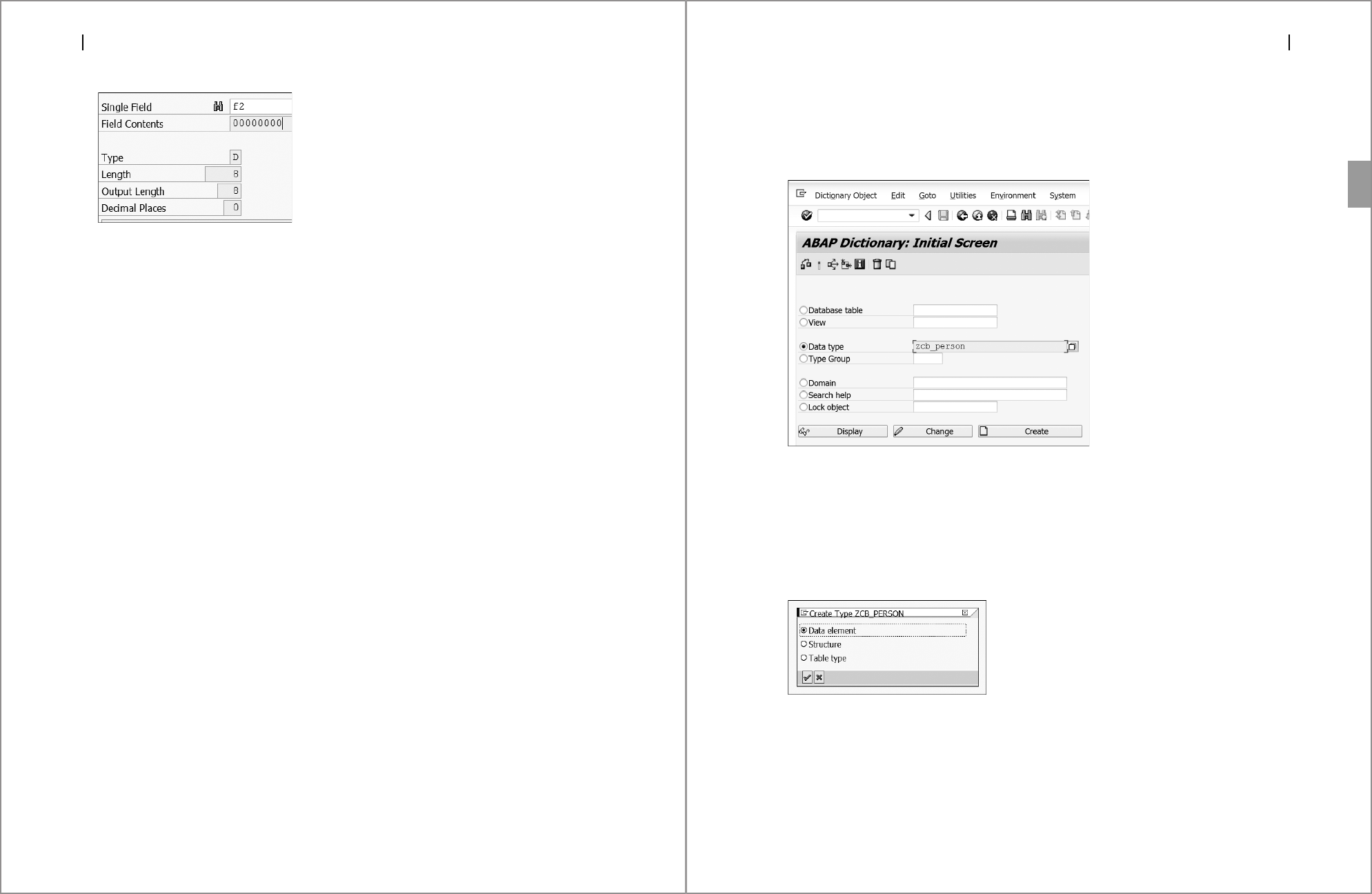
If you check the same for a data object of Type D, you’ll see that the Length and

the Output Length are the same—eight bytes—as shown in Figure 4.7.

1003 20151105 USER2

1004 20151106 USER2

Document_Number Due_Date Created_By

Table 4.5 Dates Represented in Internal Format (Cont.)

ABAP Programming Concepts

130

Figure 4.7 Output Length of Type d

If you return to Listing 4.7, you’ll see that the system outputted the date without

the separators, because there was no space in the data object to accommodate the

separators. Therefore, it simply converted the date to external format while ing-

noring the separators. The output length of each data type is predefined and can’t

be overridden manually.

If you want more control, you can create your own user-defined elementary data

types, as described earlier in this section.

4.4.2 Data Elements

As mentioned earlier, user-defined elementary data types can be created for local

reusability within the program or for global reusability across multiple programs.

The global user-defined elementary types are called data elements and are created

in ABAP Data Dictionary.

Data types defined using the

TYPE keyword are only visible within the same pro-

gram that they’re created in. If you want to create an elementary user-defined

type with global visibility across the system, you can do so in ABAP Data

Dictionary. As you may recall from Chapter 3, ABAP Data Dictionary is com-

pletely integrated into ABAP Workbench. This allows you to create and manage

data definitions (metadata) centrally.

Now, let’s create a data element in ABAP Data Dictionary. Proceed through the

following steps to create a data element

ZCB_PERSON, which is of TYPE c and

LENGTH 20:

1. Open ABAP Data Dictionary via Transaction SE11 in the command bar or by

navigating to the menu path Tools 폷 ABAP Workbench 폷 Development 폷 ABAP

Dictionary in SAP menu.

Introduction to the TYPE Concept

4.4

131

2. Select the Data Type radio button, provide a name for your data element in the

field to the right of the button, and click the Create button. Because the data

elements are repository objects, they should exist in a customer namespace

(i.e., the data element name should start with Z or Y; see Figure 4.8).

Figure 4.8 ABAP Data Dictionary: Initial Screen

3. The system presents a dialog box (see Figure 4.9) asking you to select the data

type you want to create. Data Element represents the user-defined elementary

data type, so select the Data Element radio button and click Continue (green

checkmark). (We’ll have an opportunity to explore structures and table types in

later chapters.)

Figure 4.9 Create Type

4. On the next screen (see Figure 4.10), provide a short description for your data

type to help others understand its purpose. This short text is also displayed as

a title in the (F1) help for all screen fields referring to this data element.

ABAP Programming Concepts

132

Note that the Data Type tab is selcted by default and the radio button Elemen-

tary Type preselected. Here, you have two options to maintain the technical

attributes for your data element: You can either derive them from a domain or

use one of the predefined types.

For now, use the predefined elementary data type; we’ll explore the domain

concept in the next section.

Figure 4.10 Change Data Element Screen

5. Select the Predefined Type radio button and enter the predefined type name in

the Data Type field. Note that ABAP Data Dictionary has its own predefined

elementary data types that correspond to the predefined elementary data types

in ABAP programs we discussed earlier.

6. Because we plan to create a character data type, you can enter “CHAR” in the

Data Type field or select it by using

(F4) help in the field (see Figure 4.11).

7. Enter the length of the data type in the Length field. For this data element,

enter “20”. Click the Activate button (see Figure 4.12) or press

(Ctrl)+ (F3) to

activate the data element. Save it to a package, and click Continue when an

informative message asks you to maintain field labels.

Introduction to the TYPE Concept

4.4

133

Figure 4.11 Data Type Value List

Figure 4.12 Activating a Data Element

8. If the data type supports decimals, you can also maintain the number of deci-

mal places in the Decimal Places field.

The data type we just created has global visibility and can be used to define data

objects or user-defined data types in any program, as shown:

DATA name TYPE ZCB_PERSON.

TYPES user TYPE ZCB_PERSON.

Activate Button

ABAP Programming Concepts

134

If you change the definition of the data element, the changes will be automatically

reflected for all the objects refering to that data element. This allows you to cen-

trally maintain the definitions of all related objects. Because data elements are

global objects, it’s recommended not to change them without analyzing the

impact first.

There are many things that can be maintained at the data element level, like

search helps, field labels, and help documentation. The program fields can derive

these properties automatically. We’ll explore these concepts in greater detail in

Chapter 10.

4.4.3 Domains

A domain describes the technical attributes of a field. The primary function of a

domain is to define a value range that describes the valid data values for the fields

that refer to this domain.

However, if you plan to create multiple data elements that are technically the

same, you can attach a domain to derive the technical attributes of a data element.

This allows you to manage the technical attributes of multiple data elements cen-

trally, meaning that you can change the technical attributes once for the domain,

and the change will be reflected automatically for all the data elements that use

the domain. This is an alternative to changing each individual data element to

maintain technical attributes when a predefined elementary data type is selected.

A field can’t be referred to a domain directly; it picks up the domain reference

through a data element if the domain is attached to the data element. In other

words, you always attach a domain to a data element. Figure 4.13 depicts this

relationship.

In Figure 4.13, Field 1 refers to Data Element 1, whereas Field 2 and Field 3 refer

to Data Element 2. Both Data Element 1 and Data Element 2 are using the same

domain to derive technical attributes. This implies that Field 2 and Field 3 are

both semantically and technically the same, whereas Field 1 is semantically differ-

ent from Field 2 and Field 3 but is technically the same as these two fields.

For example, a sales document number and a billing document number can both

be technically the same, such as both being ten-digit character fields. However,

the sales document and billing document are semantically different (i.e., their

purposes are different). For such a case, you can use the same domain for both the

Introduction to the TYPE Concept

4.4

135

sales document number and billing document number but a separate data ele-

ment for each.

Figure 4.13 Fields, Data Elements, and Domain Relationships

You can also maintain a conversion routine at the domain level for automatic con-

version to internal and external data formats for fields referring to a domain.

We’ll discuss this topic more in Chapter 10.

You can take a top-down approach or bottom-up approach to create a domain; that

is, you either can create the domain separately first and attach it to a data element

or can create the domain while creating the data element. Let’s take a bottom-up

approach to create a domain and attach it to the previously created data element

ZCB_PERSON.

Because domains and data elements have their own namespaces, you can use the

same name for both of them. In the following example, you’ll create a domain

using the same name as the data element created previously in Section 4.4.2; you

can use a different name if it becomes too confusing.

The following steps will walk you through the procedure to create a domain in

ABAP Data Dictionary:

1. On the initial ABAP Data Dictionary screen (Figure 4.14), select the Domain

radio button, input the name of the domain, and click the Create button.

Domains are also repository objects, so they should exist in a customer name-

space.

2. Enter a Short Description for the domain. This short description is never seen

by end users. It’s displayed when searching for domains using

(F4) help and it

helps other developers understand your domain’s purpose.

Field 1 Field 2 Field 3

Data Element 1 Data Element 2

Domain

ABAP Programming Concepts

136

Figure 4.14 ABAP Dictionary: Initial Screen

3. Use the (F4) help for the Data Type field to select the data type and enter a

value for the No. Characters field. This value defines the field length (Figure

4.15). Optionally, you can enter the number of Decimal Places for numeric

types.

Figure 4.15 Change Domain Screen

Introduction to the TYPE Concept

4.4

137

4. You can also enter Output Characteristics like output length, conversion rou-

tine, or disabling automatic uppercase conversion for screen fields referring to

this domain. We’ll explore these options further in Chapter 10.

5. Activate the domain. To attach this domain to a data element, open the data ele-

ment and select the Domain radio button under the Elementary Type radio

button, as shown in Figure 4.16. Type the name of the domain and press

(Enter).

6. Notice that the Data Type and Length are chosen by the system automatically.

If the system does not set the Data Type and Length after pressing the

(Enter)

key, it means the domain does not exist, and an informative message, No

active domain [domain_name] available, is displayed.

At this point, you can simply double-click the domain name to create it using

the top-down approach.

Figure 4.16 Attaching Domain to Data Element

4.4.4 Data Objects

Data objects derive their technical attributes from data types and occupy memory

space to store the work data of a program. ABAP statements access this content by

addressing the name of the data object. Data objects exist as an instance of data

ABAP Programming Concepts

138

types. Each ABAP data object has a set of technical attributes, such as data type,

field length, and number of decimal places.

Data objects are the physical memory units with which your ABAP statements can

work. ABAP statements can address and interpret the contents of data objects. All

data objects are declared in the ABAP program and are local to the program,

which means they exist in the program memory and can be accessed only from

within the same program. There is no concept of defining data objects centrally in

the system.

Data objects are not persistent; they exist only while the program is being exe-

cuted. The life of the data object lasts only as long as the program execution lasts.

They are created when the program execution starts and destroyed when the pro-

gram execution ends.

Before you can process persistent data (such as data from a database or a sequen-

tial file), you must read the data into data objects first, which can then be accessed

by ABAP statements. Similarly, if you want to retain the contents of a data object

beyond the end of the program, you must save it in a persistent form. Technically,

anything that can store work data in a program can be called a data object.

Let’s explore different kinds of data objects that can be defined in your ABAP pro-

grams. In the following subsections, we will look at the different classifications of

data objects.

Literals

Literals are not created using any declarative statements, nor do they have names.

They exist in the program source code and are called unnamed data objects. Like

all data objects, they have fixed technical attributes.

You cannot access the memory of a literal to read its content, because it’s an

unnamed data object. This means that literals are not reusable data objects and

their contents can’t be changed. Unlike literals, all other data objects are named

data objects, which are explicitly declared in the program.

For example, in the following snippet,

Hello World and 1234 are literals:

WRITE 'Hello World'.

WRITE 1234.

Introduction to the TYPE Concept

4.4

139

There are two types of literals:

왘

Numeric literals

Numeric literals are a sequence of digits (0 to 9) that can have a prefixed sign.

They do not support decimal separators or notation with a mantissa and expo-

nent.

Examples of numeric literals include the following:

왘

+415

왘 -345

왘 400

The following excerpt shows numeric literals used in ABAP statements:

DATA f1 TYPE I VALUE -4563.

WRITE 1234.

F1 = 1234.

왘 Character literals

Character literals are alphanumeric characters in the source code of the pro-

gram enclosed in single quotation marks (

') or back quotes (`).

For example:

'This is a text field literal'.

'1901 CA'.

`This is a string literal`.

`1901 CA`.

Character literals maintained in single quotes have the predefined type c and

length matching the number of characters. These are called text field literals.

The ones maintained with back quotes have the predefined type

string and are

called string literals. If you use character literals where a numeric value is

expected, they are converted into a numeric value. Examples of character liter-

als that can be converted to numeric types include the following:

왘

'12345'.

왘 '-12345'.

왘 '0.345'.

왘 '123E5'.

왘 '+23E+12'.

ABAP Programming Concepts

140

Variables

Variables are data objects for which content can be changed via ABAP statements.

Variables are named data objects and are declared in the declaration area of the

program. Different keywords, like

DATA and PARAMETERS, declare different types

of variables.

For now, let’s explore these two keywords, which define variables, and defer the

discussion of other keywords to later chapters.

DATA

The DATA keyword defines a variable in every context. You can use this keyword

in the global declaration area of the ABAP program to declare a global variable

that has visibility throughout the program, or you can use it inside a procedure to

declare a local variable with visibility only within the procedure—for example:

DATA field1 TYPE i

In the preceding statement, a variable with the name field1 is defined as an inte-

ger field, using the

DATA keyword.

Inline Declarations

SAP NetWeaver 7.4 introduced inline declaration, which no longer restricts you to

define your local variables separately at the beginning of the procedure. You can define

them inline as embedded in the given context, helping you to make your code thinner.

We’ll explore this concept in later chapters.

PARAMETERS

The PARAMETERS keyword plays a dual role. It defines a variable within the pro-

gram context and also generates a screen field (selection screen). This keyword is

used to create a selection screen for report programs. In these report programs,

we present a selection screen for the user to input the selection criteria for report

processing—for example:

PARAMETERS p_input TYPE c LENGTH 10.

In the preceding statement, a ten-character input field with the name p_input is

defined on the selection screen using the

PARAMETERS keyword. This field also

exists as a variable in the program and is linked to the screen field. The input

made on the selection screen for this input field will be stored in the program as

the content of the

p_input variable.

ABAP Statements

4.5

141

Constants

Constants are named data objects that are declared using a keyword and whose

content cannot be changed by ABAP statements. The keyword used to declare a

constant is

CONSTANT. It is recommended to use constants in lieu of literals wher-

ever possible. Unlike literals, constants can be reused and maintained centrally.

The syntax of constants statement mostly matches the data statement. However,

with constants statements, it is mandatory to use the addition

VALUE to assign an

initial value. This value cannot be changed at runtime. For example:

CONSTANTS c_item TYPE c LENGTH 4 VALUE 'ITEM'.

Text Symbols

A text symbol is a named data object in an ABAP program that is not declared in

the program itself. Instead, it’s defined as a part of the text elements of the pro-

gram.

A text symbol behaves like a constant and has the data type

c with the length

defined in the text element. We’ll explore text symbols further in Chapter 6.

An example of a text symbol is

WRITE text-001. In this statement, a text symbol of

the program with the number 001 is written to the output using the

WRITE state-

ment. This text symbol is defined separately in ABAP Editor via the menu path

Goto 폷 Text Elements 폷 Text Symbols.

Text symbols are accessed using the syntax

text-nnn, where nnn is the text sym-

bol number.

4.5 ABAP Statements

As we discussed earlier, the source code of an ABAP program is made up of vari-

ous ABAP statements. Unlike other programming languages like C/C++ or Java,

which contain a limited set of language-specific statements and provide most

functionality via libraries, ABAP contains an extensive set of built-in statements.

We’ll explore many ABAP statements as we progress in this book.

The best way to learn about the various ABAP statements available is to put them

in perspective with the requirements at hand. It is beyond the scope of this book

to cover all the available ABAP statements, so we’ll give a brief introduction to

ABAP Programming Concepts

142

some popular statements here, and we’ll explore these in greater detail in the

upcoming chapters:

왘

Declarative statements

Declarative statements define data types or declare data objects that are used by

the other statements in a program.

Examples include

TYPE, DATA, CONSTANTS, PARAMETERS, SELECT-OPTIONS, and

TABLES.

왘

Modularization statements

Modularization statements define the processing blocks in an ABAP program.

Processing blocks allow you to organize your code into modules. All ABAP pro-

grams are made up of processing blocks, and different processing blocks allow

you to modularize your code differently. We will explore this topic further in

Chapter 7.

Examples include the

LOAD-OF-A-PROGRAM, INITIALIZATION, AT SELECTION SCREEN,

START-OF-SELECTION, END-OF-SELECTION, AT USER-COMMAND, AT LINE-SELECTION,

GET, AT USER COMMAND, AT LINE SELECTION, FORM-ENDFORM, FUNCTION-ENDFUNC-

TION

, MODULE-ENDMODULE, and METHOD-ENDMETHOD.

왘

Control statements

Control statements control the flow of the program within a processing block.

Examples include

IF-ELSEIF-ELSE-ENDIF, CASE-WHEN-ENDCASE, CHECK, EXIT,

and

RETURN.

왘

Call statements

Call statements are used to call processing blocks or other programs and trans-

actions.

Examples include

PERFORM, CALL METHOD, CALL TRANSACTION, CALL SCREEN, SUB-

MIT

, LEAVE TO TRANSACTION, and CALL FUNCTION.

왘

Operational statements

Operational statements allow you to modify or retrieve the contents of data

objects.

Examples include

ADD, SUBTRACT, MULTIPLY, DIVIDE, SEARCH, REPLACE, CONCATE-

NATE

, CONDENSE, READ TABLE, LOOP AT, INSERT, DELETE, MODIFY, SORT, DELETE

ADJACENT

DUPLICATES, APPEND, CLEAR, REFRESH, and FREE.

Creating Your First ABAP Program

4.6

143

왘 Database access statements (Open SQL)

Database access statements allow you to work with the data in the database.

Examples include

SELECT, INSERT, UPDATE, DELETE, and MODIFY.

In this chapter thus far, we’ve explored the general program structure of an ABAP

program, learned basic rules for using ABAP syntax, touched on the use of ABAP

keywords and ABAP keyword documentation, and introduced the

TYPE concept

for data types, data elements, and data objects.

In the next section, you’ll start creating your first ABAP program using what

you’ve learned so far.

4.6 Creating Your First ABAP Program

Before we explore ABAP basics further, you’ll have the chance to create your first

program using ABAP Editor.

You’ll need developer access to the SAP system with relevant development autho-

rizations and a developer key assigned to your user ID. Contact your system

administrator if the system complains about missing authorizations or prompts

you for a developer key when creating the program.

To begin, proceed with the following steps:

1. Open Transaction SE38 or follow the menu path Tools 폷 ABAP Workbench 폷

Development 폷 ABAP Editor.

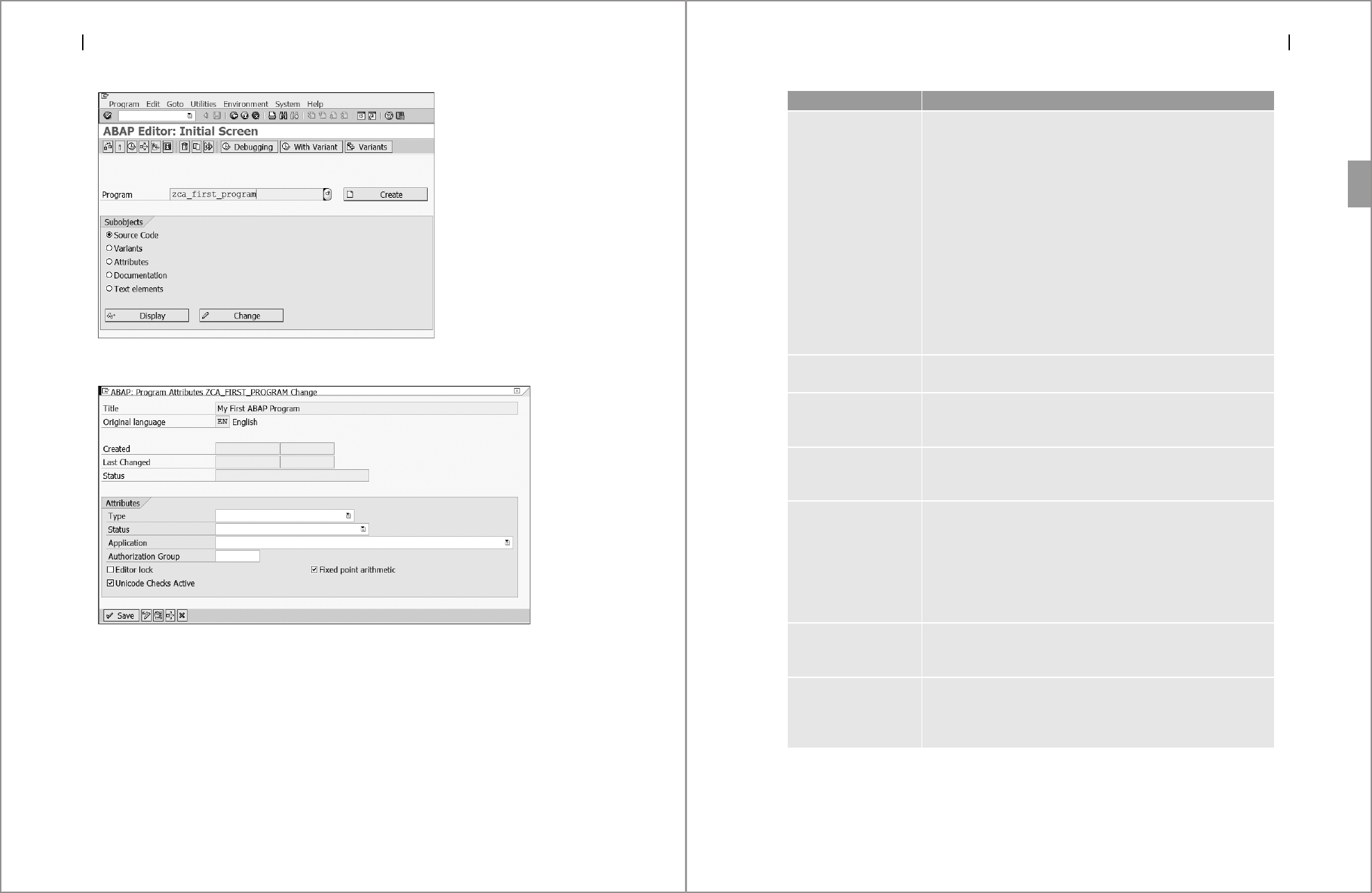
2. On the ABAP Editor initial screen, enter the program name, select the Source

Code radio button and click the Create button. Because this program will be a

repository object, it should be in a customer namespace starting with Z or Y, as

shown in Figure 4.17.

3. You’ll see the Program Attributes window (Figure 4.18) to maintain the attri-

butes for your program. Program attributes allow you to set the runtime envi-

ronment of the program.

ABAP Programming Concepts

144

Figure 4.17 ABAP Editor: Initial Screen

Figure 4.18 Program Attributes Screen

Here, you can maintain a title for your program and other attributes. The Title

and Type are mandatory fields; the others are optional.

Table 4.6 provides an explanation of all the attributes and their significance.

Creating Your First ABAP Program

4.6

145

Attribute Explanation

Type Allows you to select the type of program you wish to create.

This is the most important attribute and specifies how the pro-

gram is executed. It’s a mandatory field.

From within ABAP Editor, you can only choose from the follow-

ing program types:

왘

Executable Program

왘 Module Pool

왘 Subroutine Pool

왘 Include Program

All other program types are not created directly from within

ABAP Editor but are created with the help of special tools such

as Function Builder for function groups or Class Builder for class

pools.

Status Allows you to set the status of the program development—for

example, production program or test program.

Application Allows you to set the program application area so that the sys-

tem can allocate the program to the correct business area. For

example, SAP ERP Financial Accounting.

Authorization Group In this field, you can enter the name of a program group. This

allows you to group different programs together for authoriza-

tion checks.

Logical Database Visible only when the program type is selected as an executable

program. This attribute determines the logical database used by

the executable program. Used only when creating reports using

a logical database.

Logical databases are special ABAP programs created using

Transaction SLDB that retrieve data and make it available to

application programs.

Selection Screen Visible only when the program type is selected as an executable

program. Allows you to specify the selection screen of the logi-

cal database that should be used.

Editor Lock If you set this attribute, other users can’t change, rename, or

delete your program. Only you will be able to change the pro-

gram, its attributes, text elements, and documentation or

release the lock.

Table 4.6 Program Attributes

ABAP Programming Concepts

146

4. Under the Attributes section, provide the following values (see Figure 4.19):

왘 Type: Executable program

왘 Status: Test Program

왘 Application: Unknown application

왘 Also check the Unicode Checks Active and Fixed point arithmetic check-

boxes.

Click the Save button when finished.

Figure 4.19 Maintaining Program Attributes

Fixed Point Arithmetic If this attribute is set for a program, the system rounds type p

fields according to the number of decimal places, or pads them

with zeros.

The decimal sign in this case is always the period (

.), regardless

of the user’s personal settings. SAP recommends that this attri-

bute is always set.

Unicode Checks Active This attribute allows you to set if the syntax checker should

check for non-Unicode-compatible code and display a warning

message.

As of SAP NetWeaver 7.5, the system does not support non-

Unicode systems, so this option is always selected by default.

Start Using Variant Applicable only for executable programs. If you set this attri-

bute, other users can only start your program using a variant.

You must then create at least one variant before the report can

be started.

Attribute Explanation

Table 4.6 Program Attributes (Cont.)

Creating Your First ABAP Program

4.6

147

5. On the Create Object Directory Entry screen (see Figure 4.20), you can assign

the program to a package. The package is important for transports between sys-

tems. All of the ABAP Workbench objects assigned to one package are com-

bined into one transport request.

When working in a team, you may have to assign your program to an existing

package, or you may be free to create a new package. All programs assigned to

the package

$TMP are private objects (local object) and can’t be transported into

other systems. For this example, create the program as a local object.

Figure 4.20 Assigning Package

6. Either enter “$TMP” as the Package and click the Save button or simply click

the Local Object button (see Figure 4.20).

7. This takes you to the ABAP Editor: Change Report screen where you can write

your ABAP code. By default, the source code includes the introductory state-

ment to introduce the program type. For example, executable programs are

introduced with the

REPORT statement, whereas module pool programs are

introduced with the

PROGRAM statement.

8. Write the following code in the program and activate the program:

PARAMETERS p_input TYPE c LENGTH 20.

WRITE : 'The input was:', p_input.

9. In the code, you’re using two statements—PARAMETERS and WRITE. The PARAME-

TERS

statement generates a selection screen (see Figure 4.21) with one input

field. The input field will be of

TYPE c with LENGTH 20, so you can input up to

twenty alphanumeric characters.

ABAP Programming Concepts

148

Here, the PARAMETERS statement is performing a couple of tasks:

왘 Declaring a variable called

p_input.

왘 Generating a screen field (screen element) on the selection screen with the

same name as the variable

p_input. The screen field p_input is automati-

cally linked to the variable sharing the same name. Therefore, the data

transfer between the screen and the program is handled automatically. In

other words, if you enter some data in the

p_input screen field, it will be

automatically transferred to the program and stored in the

p_input vari-

able. This data in the

p_input variable can then be accessed by other state-

ments, like you’re doing with the

WRITE statement to print it in the output.

Figure 4.21 Selection screen

10. Enter a value in the input field and click the Execute button, or press (F8). This

should show you the output or List screen, as shown in Figure 4.22.

Figure 4.22 List Screen

11. The list screen (output screen) is generated by the WRITE statement in the code.

With the

WRITE statement, you’re printing the contents of two data objects

Summary

4.7

149

here. One is a text literal, 'The input was:', and the other is the variable p_

input

created by the PARAMETERS keyword.

Whatever input was entered on the selection screen was transferred to the

program and stored in the variable

p_input, which was then processed by the

WRITE statement to display in the output.

We’ll have many opportunities to work with different types of screens as we

progress through the book.

4.7 Summary

In this chapter, you learned the basics of the ABAP programming language ele-

ments. You saw that ABAP programs can only work with data of the same pro-

gram. Because we typically process various kinds of data in the real world, we

explained the different elementary types that are supported by the system to pro-

cess various kinds of data. Because the basic task of an ABAP program is to pro-

cess data, this understanding is crucial to process the data consistently.

We also described the syntax to write a couple of statements. We’ll explore more

statements as we progress through the book. In the final section, you created your

first ABAP program.

By now, you should have a good understanding of data types and data objects.

However, if you find yourself a little lost, don’t worry; the concepts should make

more sense as we work through creating more programs in the next chapter. In

the next chapter, we’ll discuss complex data types and internal tables.

305

Chapter 8

Some elements of ABAP programs can be designed using procedural or

object-oriented programming. This chapter explores the concepts of object-

oriented programming and their implementation in ABAP.

8 Object-Oriented ABAP

ABAP is a hybrid programming language that supports both procedural and

object-oriented programming (OOP) techniques. In this chapter, we’ll discuss the

various concepts used in OOP and the advantages it provides over procedural

programming techniques.

We’ll start with a basic overview of OOP in Section 8.1. This introduction should

help you appreciate the advantages of using OOP techniques. To understand

OOP, you’ll need to understand concepts such as encapsulation, inheritance,

polymorphism, data encapsulation, and information hiding. We’ll start examin-

ing those concepts in Section 8.2 with a look at encapsulation and the techniques

to hide implementation from the outside world.

In Section 8.3, we’ll discuss inheritance and the techniques that allow you to

leverage existing features and functionality without having to reinvent the wheel.

In Section 8.4, we’ll look at polymorphism, which allows the same object to

behave differently at runtime. We’ll conclude the chapter with a discussion of

XML in Section 8.5.

8.1 Introduction to Object-Oriented Programming

Before OOP, everything was based on functions and variables without focusing

on the object itself. With OOP, the focus is on objects, which represent real-life

entities, with functions and variables approximating the objects.

Traditional programming focused on developing programming logic to manipu-

late data—for example, a logical procedure that takes input data, processes it, and

Object-Oriented ABAP

306

produces output. However, OOP focuses on the object being manipulated rather

than the logic to manipulate the data.

If you look around, you’ll see many real-world objects, such as your car, your

dog, your laptop, and so on. Each of these real-world objects is represented as a

software object in OOP. Real-world objects have two characteristics: states and

behaviors. For example, a car has states such as its current gear, current speed,

and so on, and behaviors such as changing gears, applying brakes, and so on. Soft-

ware objects that represent real-world objects also have states and behaviors;

software objects store their states in variables (called attributes) and contain func-

tions (called methods) to manipulate or expose the states of the object. For exam-

ple, a car object can have attributes to store the current speed, current gear, and

so on, and methods to read the current speed or change the gear.

Methods operate on the internal state of the object; that is, they can access the

attributes of their own object and serve as a mechanism for communication

between objects. Hiding this internal state of the object and routing all access to

the object through its methods is known as encapsulation. Encapsulation is a fun-

damental principle of OOP, which we’ll discuss in Section 8.2.

Sometimes, an object may share many similarities with other objects while hav-

ing specific features of its own. For example, a mountain bike may have all the

features of a road bike plus certain features unique only to mountain bikes. The

concept of inheritance helps us leverage existing code and avoid code redundancy

while extending functionality. We’ll discuss inheritance in Section 8.3.

Identifying the states and behaviors of real-world objects is the first step to start

thinking in terms of OOP. Before exploring OOP further, let’s consider a simple

procedural programming application that calculates a person’s body mass index

(BMI). We’ll then look at how this application can be designed using OOP. For

this example, we can create a function module with three interface parameters:

height, weight, and BMI. We can pass the person’s height and weight to the func-

tion and receive the calculated BMI as a result, as shown in Listing 8.1.

FUNCTION ZCALCULATE_BMI.

*"---------------------------------------------------------------

*"*"Local Interface:

*" IMPORTING

*" REFERENCE(HEIGHT) TYPE I

*" REFERENCE(WEIGHT) TYPE I

*" EXPORTING

Introduction to Object-Oriented Programming

8.1

307

*" REFERENCE(BMI) TYPE I

BMI = WEIGHT / HEIGHT.

ENDFUNCTION.

Listing 8.1 Example Function Module to Calculate BMI

Listing 8.2 shows the call to the function module zcalculate_bmi that we defined

in Listing 8.1.

REPORT ZCA_BMI.

DATA : v_bmi TYPE I.

PARAMETERS: p_height TYPE I,

P_weight TYPE I.

CALL FUNCTION 'ZCALCULATE_BMI'

EXPORTING

height = p_height

weight = p_weight

IMPORTING

bmi = v_bmi.

WRITE: 'Your BMI is', v_bmi.

Listing 8.2 Program to Calculate BMI

When the function module is called in the program, the whole function group to

which this function module belongs is loaded into the memory (internal session)

the main program is assigned to. Each subsequent call to this function module in

the program will access the existing instance in the memory as opposed to load-

ing a new instance.

When a function module is called in a program, one instance of it is created in the

internal session in which the program runs, and each subsequent call to this func-

tion module from the program will point to the existing instance that was previ-

ously loaded into the internal session. You can’t have multiple instances of the

same function module within the same internal session.

If you call the

zcalculate_bmi function module in the program to calculate the

BMI of multiple persons, there’s no way for the function module to be aware of

the person for which the BMI is calculated. You can define a global variable in the

function group to store a person’s name so that other function modules of the

function group can use this information, but it’s easy to lose track of all these vari-

ables in the code—and even then, this design can only support one person at a

time in the application.

Object-Oriented ABAP

308

The focus of the function module here is to take a certain input and process it to

produce a result. OOP shifts the focus to the object. In this example, we define an

object that represents a person and then define attributes and methods to store

and process the person’s BMI.

In this section, we’ll look at the defining elements of OOP, including classes,

methods, instances and static components, and events.

8.1.1 Classes

Objects encapsulate data and create functions to manipulate that data. The charac-

teristics (called attributes) and functions (called methods) of an object are put into

one package. The definition of this package is called a class. To use objects in a

program, classes must be defined, because an object exists as an instance of a

class.

A class can be defined as shown in Listing 8.3.

REPORT ZCA_BMI.

CLASS CL_PERSON DEFINITION.

PUBLIC SECTION.

TYPES ty_packed TYPE p LENGTH 4 DECIMALS 2.

METHODS set_height IMPORTING im_height TYPE ty_packed.

METHODS set_weight IMPORTING im_weight TYPE ty_packed.

METHODS set_bmi.

METHODS get_bmi RETURNING VALUE(r_bmi) TYPE ty_packed.

PRIVATE SECTION.

DATA : bmi TYPE I,

height TYPE I,

weight TYPE I.

ENDCLASS.

CLASS CL_PERSON IMPLEMENTATION.

METHOD set_height.

height = im_height.

ENDMETHOD.

METHOD set_weight.

weight = im_weight.

ENDMETHOD.

METHOD set_bmi.

bmi = height / weight.

ENDMETHOD.

METHOD get_bmi.

r_bmi = bmi.

ENDMETHOD.

ENDCLASS.

Introduction to Object-Oriented Programming

8.1

309

DATA john TYPE REF TO cl_person.

DATA mark TYPE REF TO cl_person.

START-OF-SELECTION.

CREATE OBJECT john.

john->set_height( exporting im_height = 165 ).

john->set_weight( exporting im_weight = 50 ).

john->set_bmi( ).

WRITE : / 'John’s BMI is', john->get_bmi( ).

CREATE OBJECT mark.

mark->set_height( exporting im_height = 175 ).

mark->set_weight( exporting im_weight = 80 ).

mark->set_bmi( ).

WRITE : / 'Mark’s BMI is', mark->get_bmi( ).

IF john->get_bmi( ) GT mark->get_bmi( ).

WRITE : / 'John is fatter than Mark'.

ELSE.

WRITE : / 'Mark is fatter than John'.

ENDIF.

Listing 8.3 Using Objects

A class consists of two sections: a definition section and an implementation sec-

tion. In the definition section, we define the components of the class, such as attri-

butes, methods, and events. The attributes of a class store the state of an object,

and the methods implement the logic to manipulate the behavior of an object by

accessing the attributes.

Different events can be defined for the class, which can be raised during the run-

time of the object. Methods can be called directly or can respond to events

defined in the class. In the implementation section, we implement the methods to

manipulate the behavior of an object or to respond to the events of the class.

Each class component can belong to a specific visibility section, such as public,

protected, or private. The visibility section enables data encapsulation by putting

restrictions on how the class component can be accessed. For example, a compo-

nent belonging to the public visibility section can be accessed by external objects

and programs without any restrictions, whereas a component belonging to the

private visibility section can be accessed only by the methods of the same class.

Object-Oriented ABAP

310

Components belonging to the protected section can be accessed by the methods

of the same class and its subclasses. A subclass inherits its components from a par-

ent class. Once a class inherits from a parent class, it can access the public and

protected components of the parent class. We’ll learn more about encapsulation

in Section 8.2.

In Listing 8.3, we defined the

CL_PERSON class consisting of HEIGHT, WEIGHT and

BMI attributes in the private visibility section. Because these attributes are private,

they can’t be accessed by external objects or programs directly. To manipulate

these attributes, we defined setter and getter methods in the public section of the

class. Setter methods allow you to set the value of an attribute, and getter methods

allow you to read the value of an attribute. Defining the attributes in the private

section and providing setter and getter methods to manipulate the attributes

allows for more control, such as validating the data before changing the state of

the object.

For example, we can avoid an invalid value being set for a person’s height by val-

idating the input in the

SET_HEIGHT method. In the program, we defined two

object reference variables called

JOHN and MARK referring to the CL_PERSON class. An

object exists as an instance of a class, and each class can have multiple instances.

The object reference variable initially contains an empty value until the object is

instantiated using the

CREATE OBJECT statement. Once the object is instantiated,

the object reference variable contains the reference (pointer) to the object in

memory, and the object is accessed using the object reference variable. The object

reference variables are also called reference objects and are defined using the

TYPE

REF

TO addition.

Unlike in function modules, here each reference object occupies its own memory

space and multiple instances of the class can be defined in the program, with each

instance working with its own data.

In this section, we’ll discuss local and global classes, class parts and components,

and the use of visibility in classes.

Local and Global Classes

As previously discussed, classes can be defined locally in an ABAP program or

globally in the system using Class Builder (Transaction SE24). Local classes can be

used only within the program in which they’re defined, whereas global classes can

Introduction to Object-Oriented Programming

8.1

311

be used in any ABAP program. Irrespective of whether the class is defined locally

or globally, the syntax to define the class remains the same, as shown in Listing

8.3. Apart from visibility, there is no difference between a local class and a global

class. When a class is used in an ABAP program, the system first searches if the

class exists locally. If the class isn’t defined locally, then the system looks for a

global class.

When defining global classes, we can use the form-based editor of the Class

Builder tool to easily define the components of the class and implement the meth-

ods without getting into the nitty gritty of the syntax.

Wherever applicable, we will show you the steps to define classes both locally

and globally throughout this chapter. Define local classes if the scope of the object

is limited to the program and the object may be irrelevant to other programs, but

if you plan to use an object in multiple programs, we recommend defining the

class globally in Class Builder.

Class Parts and Components

To break down the code in Listing 8.3 further, a class in ABAP has two sections:

왘

Definition section

In the definition section, various components of a class, such as attributes,

events, and methods, are defined. For example, in Listing 8.3, we defined the

attributes and the methods of the class in the definition section of the class.

When defining the methods, we also defined the parameter interface for the

methods.

For the sake of simplicity, we haven’t defined any events in Listing 8.3, but if

you want to trigger various events to which the methods of the class can

respond, you can do so in the definition part of the class. The methods that

respond to events are called event handler methods. We’ll learn more about

defining events and implementing suitable event handler methods in Section

8.1.4.

왘

Implementation section

The implementation section of the class is where we implement the methods

defined in the definition section. The methods are implemented between the

METHOD and ENDMETHOD statements, and each method defined in the definition

part must have an implementation in the implementation part of the class.

Object-Oriented ABAP

312

There are three important types of components available in a class:

왘

Methods

Methods are used to change the state of an object and manipulate its behavior.

For example, in Listing 8.3, different methods were implemented in the

CL_

PERSON

class to set the height, weight, and BMI of the person. Methods can also

be defined as event handler methods that respond to specific events during the

runtime of the object. By using setter and getter methods, we can ensure that

all attributes of the class are always accessed through its methods, thus guaran-

teeing data consistency.

왘

Attributes

Attributes are the internal data fields of a class and store the state of an object.

We can change the state of an object by changing the contents of an attribute.

왘

Events

Events are defined in the definition area of a class and can be raised during the

runtime of the object. A suitable event handler method is maintained in the

implementation part of the class and is triggered when the corresponding event

is raised. Events allow you to call specific methods dynamically during the run-

time of the object.

For example, if you want to perform specific tasks when the user double-clicks

an output line, you can maintain a

DOUBLE_CLICK event, which can be raised on

that event. The registered event handler method will be called dynamically

when the event is raised.

The components of a class can be categorized as follows:

왘

Static components

Static components can be accessed directly using the class component selector

=>. Static components behave similarly to function modules in that only one

instance of a static component exists in the program.

왘

Instance components

Instance components can’t be accessed directly using the class name. To access

an instance component, you need to define a reference object in the program

using TYPE REF TO (for example, the objects John and Mark in Listing 8.3) and

then access its attributes and methods through the reference object using the

object component selector

->.

Introduction to Object-Oriented Programming

8.1

313

Before the attributes and methods can be accessed through the reference

object, the reference object needs to be instantiated using the

CREATE OBJECT

statement, which creates an instance of the class (an object described by the

class) in the program.

We’ll discuss static and instance components further in Section 8.1.3.

Visibility

The components of a class can have different visibility sections, such as public,

protected, and private. The visibility is set in the definition part of the class. Com-

ponent visibility allows for data encapsulation and hiding the implementation

from the external world.

Encapsulation is an important concept in OOP, and we’ll discuss visibility further

in Section 8.2.

8.1.2 Methods

A method can access other components of the same object. To access the attributes

and methods of the same class, a special self-reference variable,

me, is used. Even

though the components of the class can be accessed directly from within the

methods of the same class, for better readability it’s recommended to use the self-

reference variable

me when accessing the same class components. You can access

both static and instance components from within an instance method, whereas

you only can access static components from within a static method.

To call a method of the class, we can either use the

CALL METHOD statement (e.g.,

CALL METHOD John->get_bmi) or use the object component selector and parenthe-

ses directly (e.g.,

john->get_bmi( )).

A method can have importing, exporting, changing, and returning parameters.

The importing, exporting, and changing parameters behave similarly to the pa-

rameters we define in function modules. For example, data is imported through

importing parameters and exported through exporting parameters, while chang-

ing parameters can be used for both importing and exporting.

The methods that use returning parameters are called functional methods. Prior to

SAP NetWeaver 7.4, functional methods could only have one returning parameter

and no exporting parameters. However, with SAP NetWeaver 7.4, this restriction

Object-Oriented ABAP

314

is lifted. Functional methods are typically used when a result is returned to the

caller program that can be directly assigned to a data object in the program.

For example, with the statement

v_bmi = oref->get_bmi( ), v_bmi is the data

object,

oref is the reference object, and get_bmi is a method with a returning

parameter the value of which will be assigned to the

v_bmi variable.

Inheritance

Often, many objects are different, but similar enough to be put into a single class.

For example, animals and humans have heartbeats, so a class may have a

get_

heart_beat

method. However, dogs have tail lengths, so should this class also

have a

get_tail_length method? No, we can define another class as a child class

(called a subclass) of the parent class. This subclass will have all the features of the

parent class plus some additional features. This allows you to extend the function-

ality of your applications while leveraging the existing code.

Let’s look at an example. Objects are designed to closely represent real-life

objects—such as a printer. A printer may have an external interface, including a

paper tray, keypad, and so on, and the basic functionality of the printer is to cre-

ate a printout. OOP objects can be designed to represent that setup.

Therefore, let’s create a class called

printer with a method called print, as shown

in Listing 8.4.

CLASS PRINTER DEFINITION.

PUBLIC SECTION.

METHODS print.

ENDCLASS.

CLASS PRINTER IMPLEMENTATION.

METHOD print.

WRITE 'document printed'.

ENDMETHOD.

ENDCLASS.

Listing 8.4 Parent Class for Printer

This is a basic printer, but what if we want to extend its functionality? For exam-

ple, if we have a new printer model that has a counter feature to keep track of the

number of copies printed, do we have to build all of the printer logic from

scratch? No, we can define a subclass, as shown in Listing 8.5, that inherits all the

functionality of the basic printer and extends it.

Introduction to Object-Oriented Programming

8.1

315

CLASS PRINTER_WITH_COUNTER DEFINITION INHERITING FROM PRINTER.

PUBLIC SECTION.

DATA counter TYPE I.

METHODS print REDEFINITION.

ENDCLASS.

CLASS PRINTER_WITH_COUNTER IMPLEMENTATION.

METHOD print.

Counter = counter + 1.

CALL METHOD SUPER->PRINT.

ENDMETHOD.

ENDCLASS.

Listing 8.5 Subclass Implementation

In Listing 8.5, the class PRINTER_WITH_COUNTER is inherited from the class printer.

Here,

printer is the superclass (parent class) and PRINTER_WITH_COUNTER is the

subclass (child class). This process of a subclass inheriting the traits of a superclass

is called inheritance in OOP.

Notice the keyword

INHERITING FROM used in the definition of the class PRINTER_

WITH_COUNTER

. The subclass inherits all the components of the parent class. It will,

by default, have all the attributes and methods defined in the parent class. If

required, the methods inherited in the subclass can be redefined to add function-

ality.

In Listing 8.5, the

print method in the PRINTER_WITH_COUNTER subclass is rede-

fined to increment the counter attribute and calls the

print method of the parent

class. This effectively extends the functionality of the method while leveraging

the existing functionality provided by the method of the parent class. Because the

same

print method behaves differently in the superclass and subclass, it leads to

some interesting behavior called polymorphism (meaning having many forms),

which we’ll discuss in Section 8.4.

Now we have a printer with a counter, and we know that the counter increments

by one every time a document is printed. However, what will its initial value be?

How do we ensure that the counter always starts from one or any other initial

value? These details are sorted out by defining a constructor for the class.

There are two types of constructors:

왘

Instance constructor

An instance constructor is a special method called when the object is instanti-

ated. The instance constructor is called for each object when it is instantiated.

Object-Oriented ABAP

316

왘 Class constructor

The class constructor is special method called just once for the whole class in one

internal mode. A class constructor can have a maximum of one instance and

one static constructor. A static constructor can’t have any parameters, whereas

the instance constructor can have only importing parameters.

By defining importing parameters for the instance constructor, we can ensure

that the object is always initialized before any of its attributes or methods are

accessed.

Listing 8.6 shows the implementation of the constructor.

CLASS PRINTER_WITH_COUNTER DEFINITION INHERITING FROM PRINTER.

PUBLIC SECTION.

DATA counter TYPE I.

METHODS constructor IMPORTING count TYPE I.

METHODS print REDEFINITION.

ENDCLASS.

CLASS PRINTER_WITH_COUNTER IMPLEMENTATION.

METHOD constructor.

CALL METHOD super->constructor.

counter = count.

ENDMETHOD.

METHOD print.

counter = counter + 1.

CALL METHOD SUPER->PRINT.

ENDMETHOD.

ENDCLASS.

START-OF-SELECTION.

DATA oref TYPE REF TO PRINTER_WITH_COUNTER.

CREATE OBJECT oref

EXPORTING

count = 0.

Listing 8.6 Class with Constructor

In Listing 8.6, the constructor method is defined in the definition part of the

PRINTER_WITH_COUNTER class with one importing parameter, count. Because the

PRINTER_WITH_COUNTER class is a subclass of the printer class, the superclass con-

structor must be called first in the implementation of the constructor method,

even if there’s no constructor defined in the superclass. This ensures that all of

the superclass components in the inheritance tree are initialized properly. If a

constructor is defined in the superclass, it won’t be inherited by the subclass. This

Introduction to Object-Oriented Programming

8.1

317

allows each class in the inheritance tree to have its own constructor in order to

initialize its attributes per requirements.

In the example in Listing 8.6, the

count parameter of the constructor is assigned

a value when instantiating the reference object

oref. The syntax checker will give

an error if the constructor’s mandatory parameters aren’t passed while instantiat-

ing the reference object. This ensures that the object is always instantiated prop-

erly.

Now, say we have a more advanced printer model that can print multiple copies

along with the basic features provided so far. To create this printer, we’ll inherit

the

PRINTER_WITH_COUNTER class and add additional functionality, as shown in Lis-

ting 8.7.

CLASS MULTI_COPY_PRINTER DEFINITION INHERITING FROM PRINTER_WITH_

COUNTER.

PUBLIC SECTION.

DATA copies TYPE I.

METHODS set_copies IMPORTING copies TYPE I.

METHODS print REDEFINITION.

ENDCLASS.

CLASS MULTI_COPY_PRINTER IMPLEMENTATION.

METHOD set_copies.

Me->copies = copies.

ENDMETHOD.

METHOD print.

Do copies TIMES.

CALL METHOD SUPER->Print.

ENDDO.

ENDMETHOD.

ENDCLASS.

START-OF-SELECTION.

DATA oref TYPE REF TO MULTI_COPY_PRINTER.

CREATE OBJECT oref

EXPORTING

count = 0.

oref->set_copies( 5 ).

oref->print( ).

Listing 8.7 Class Extended to Print Multiple Copies

In Listing 8.7, we defined the MULTI_COPY_PRINTER class, inheriting from PRINT-

ER_WITH_COUNTER.

In the MULTI_COPY_PRINTER class, we defined a method called

Object-Oriented ABAP

318

set_copies that receives the copies importing parameter and assigns the value to

the

copies attribute. We redefined the print method to print multiple copies by

calling the method in the superclass in a

DO loop.

It’s good practice not to allow direct access to the class attributes and to use meth-

ods to set or get attribute values. This gives us more control while manipulating

attributes. The methods that set values are called setter methods and the methods

that are used to get values are called getter methods. Setter methods are prefixed

with

set_ and getter methods are prefixed with get_.

Encapsulation

Now, say our printer is an industrial printer and we want to set a restriction for

the minimum number of prints. For example, the printer should only take a

request if a minimum of fifty copies is requested. We implement this restriction

by writing an

IF condition in the set_copies method, as shown in Listing 8.8.

METHOD set_copies.

IF copies GE 50.

Me->copies = copies.

ELSE.

*Raise exception

ENDIF.

ENDMETHOD.

Listing 8.8 Restricting Copies in set_copies Method

The code in Listing 8.8 adds the restriction to set the copies attribute only if the

value is greater than or equal to 50. However, there’s one loophole in this imple-

mentation: Because the

copies attribute is defined with its visibility as public,

anyone can directly access this attribute from outside the class and set a value,

thus bypassing the check in the

set_copies method, as shown in Listing 8.9.

DATA oref TYPE REF TO MULTI_COPY_PRINTER.

CREATE OBJECT oref

EXPORTING

count = 0.

oref->copies = 5.

oref->print( ).

Listing 8.9 Bypassing set_copies Method to Set Number of Copies

As you can see in Listing 8.9, we can directly access the copies attribute to set the

number of copies. This is where encapsulation and implementation hiding plays an

Introduction to Object-Oriented Programming

8.1

319

important role. By defining clear boundaries on what can be accessed from out-

side the class and what should be restricted, we not only make it easy for devel-

opers to use our classes, because they only need to know the public interface

(components that are publicly accessible) of our class, but also ensure that inad-

vertent bugs don’t creep into our software implementation.

Encapsulation also gives you the freedom to change the private sections of the

class according to changing requirements without having to worry about depen-

dencies. For example, if you change the interface of a method in the public visi-

bility section, all the programs that call this method will be affected; however,

because no programs can directly access the private section of a class, you can

change private sections freely without having to worry about program dependen-

cies.

In this example, we can make the attribute

copies private so that it can be ac-

cessed only from the methods of the same class, as shown in Listing 8.10.

CLASS MULTI_COPY_PRINTER DEFINITION INHERITING FROM PRINTER_WITH_

COUNTER.

PUBLIC SECTION.

METHODS set_copies IMPORTING copies TYPE I.

METHODS print REDEFINITION.

PRIVATE SECTION.

DATA copies TYPE I.

ENDCLASS.

Listing 8.10 Making Attribute Private

As you can see, we made our printer more and more complex without having to

duplicate any code. Also, as the printer added advanced capabilities, it still per-

formed the basic task of printing a document. Therefore, a user using the

advanced model of the printer need not be aware of its advanced features to per-

form the basic task of printing a document. This is similar to a car with advanced

features like cruise control. The driver need not know how to set cruise control to

drive the car, but he can learn to set cruise control to take advantage of it.

In addition, if the

print method in the printer superclass is enhanced, then all

the enhancements will be available by default to all the subclasses without having

to change any of them.

Object-Oriented ABAP

320

8.1.3 Instance and Static Components

A class can contain both instance and static components. An instance attribute

can have multiple instances in the program, whereas a static attribute has only

one instance. An instance component is accessed through a reference object using

the object component selector

->, whereas a static component is accessed using

the class component selector

=>. Static components are preceded by the CLASS

keyword during the definition.

Listing 8.11 shows the definition of both instance and static components. For

simplicity, we’re accessing the attributes of the class directly in this example, but

in real-world code direct access to attributes should always be avoided by using

setter and getter methods.

CLASS CL_PERSON DEFINITION.

PUBLIC SECTION.

CLASS-DATA height TYPE I. "Static attribute

DATA weight TYPE I. "Instance attribute

METHODS get_bmi EXPORTING bmi TYPE I. "Instance method

METHODS constructor "Instance constructor

IMPORTING name TYPE CHAR20.

CLASS-METHODS set_height "Static Method

IMPORTING height TYPE I.

CLASS-METHODS class_constructor. "Static Constructor

ENDCLASS.

CLASS CL_PERSON IMPLEMENTATION.

METHOD class_constructor.

ENDMETHOD.

METHOD constructor.

ENDMETHOD.

METHOD get_bmi.

ENDMETHOD.

METHOD set_height.

ENDMETHOD.

ENDCLASS.

DATA oref TYPE REF TO cl_person. "Defining reference object

DATA v_bmi TYPE I.

START-OF-SELECTION.

*Accessing static attributes and methods using the selector "=>"

*with class reference

cl_person=>height = 165.

CALL METHOD cl_person=>set_height

EXPORTING

height = 165.

*Instantiating the reference object and accessing the instance

Introduction to Object-Oriented Programming

8.1

321

*attributes and methods using the selector "->" with object

*reference.

CREATE OBJECT oref

EXPORTING

name = 'JOHN'.

oref->weight = 50.

CALL METHOD oref->get_bmi

IMPORTING

bmi = v_bmi.

Listing 8.11 Instance and Static Class Components

As shown, static components are defined with the preceding keyword CLASS (e.g.,

CLASS-DATA, CLASS-METHODS) and accessed using the => selector with the class

name reference directly (e.g.,

class_name=>component). Static methods are some-

what similar to function modules in that only one instance exists in the program

memory and each subsequent call to the method points to the same instance,

whereas each reference object works with its own instance components.

A static constructor can’t have any parameter interface, whereas an instance con-

structor can have importing parameters. A static constructor is executed only

once on the first access of any of the class components, including instantiation of

any reference object. An instance constructor is executed each time a reference

object is instantiated.

Table 8.1 compares and contrasts instance and static components.

Instance Component Static Component

Instance components are accessed through

a reference object with the

-> selector.

Static components can be accessed directly

through the class name reference with the

=> selector even before a reference object

is instantiated. They can also be accessed

using a reference object.

Multiple instances can exist. Only single instance exists.

Within an instance method, both static and

instance attributes can be accessed.

Within a static method, only static attri-

butes or static methods can be accessed.

To access the instance components of a

class, a reference object needs to be

defined in the program and instantiated

using CREATE OBJECT statement.

Static components can be accessed directly

from program using a class reference (simi-

lar to calling a function module directly)

without the need for a reference object.

Table 8.1 Differences between Instance and Static Components

Object-Oriented ABAP

322

8.1.4 Events

Events can be defined in a class to be triggered from a method (called triggers)

when a specific event takes place during the runtime of the object; specific meth-

ods (called event handlers) react to these events. For example, we can define an

event called

double_click in the class to be triggered in one of the methods when

the user double-clicks the report output. The

on_double_click method can be

defined as an event handler for this event so that it’s executed when the

double_

click

event is triggered from the trigger method.

To trigger an event, the class must have the events defined in the definition part

of the code and triggered in one of its methods. Instance events are defined using

the

EVENTS keyword and static events are defined using the CLASS-EVENTS key-

word. A static event can be triggered from both static and instance methods,

whereas, an instance event can only be triggered from an instance method.

Events can have exporting parameters that are passed to the event handler

method when the event is triggered. To trigger an event, the statement

RAISE

EVENT

event_name is used in one of the methods of the class. The EXPORTING addi-

tion is used with the

RAISE EVENT keyword to pass the event parameters to the

event handler method.

Event handlers are special methods that are defined to react to the event. Event

handler methods are defined in the definition part of the class as methods for spe-

cific events. The syntax to define an event handler method is

METHODS method_

name

FOR EVENT event_name OF class_name, where method_name is the name of the

event handler method,

event_name is the name of the event, and class_name is

the name of the class in which the event is defined. If the event has exporting

An instance constructor only can have

importing parameters and is executed each

time a reference object is instantiated.

A static constructor can’t have any parame-

ter interface and is executed only once per

program session. However, it’s executed

before the instance constructor, if the class

has both static and instance constructors,

and when the first reference object is

instantiated, provided it isn’t loaded previ-

ously.

Instance Component Static Component

Table 8.1 Differences between Instance and Static Components (Cont.)

Introduction to Object-Oriented Programming

8.1

323

parameters defined, then the event handler must import all non-optional param-

eters. All instance events have an implicit

sender parameter that can be imported

in the event handler. The

sender parameter contains a reference to the sender

object in which the event is defined. To define a static method as an event han-

dler, use the CLASS-METHODS keyword.

To allow an event handler method to react to an event, we must determine at run-

time the trigger to which it is to react. We can do that by using the

SET HANDLER

statement. The SET HANDLER statement registers the event handler methods with

the event triggers.

Instance events can be registered to a specific instance or to all instances, whereas

static events are registered to the whole class. The syntax to use

SET HANDLER state-

ment for instance events is as follows:

SET HANDLER event_handler_method FOR oref.

or:

SET HANDLER event_handler_method FOR ALL INSTANCES.

The syntax to use the SET HANDLER statement for static events is as follows:

SET HANDLER event_handler_method.

Here, event_handler_method is an instance or static method that is defined as an

event handler for an event. The event handler method will not be triggered if the

handler is not registered using the SET HANDLER statement.

Listing 8.12 shows an example to define and register events in a class. This exam-

ple defines the

cl_events_demo class with two events, double_click and right_

click

. Here, double_click is defined as an instance event and right_click is

defined as a static event. The

double_click event also has a couple of mandatory

exporting parameters (

column and row) defined. We’ve also defined a trigger_

event

method to act as a trigger method. This is defined similarly to any regular

method. The

on_double_click and on_right_click methods are defined as event

handler methods for the

double_click and right_click events, respectively.

CLASS cl_events_demo DEFINITION.

PUBLIC SECTION.

EVENTS double_click

EXPORTING

VALUE(column) TYPE i

VALUE(row) TYPE i .

CLASS-EVENTS right_click .

Object-Oriented ABAP

324

METHODS trigger_event.

METHODS on_double_click FOR EVENT double_click OF cl_events_demo

IMPORTING

column

row

sender.

METHODS on_right_click FOR EVENT right_click OF cl_events_demo.

ENDCLASS.

CLASS cl_events_demo IMPLEMENTATION.

METHOD trigger_event.

RAISE EVENT double_click

EXPORTING

column = 4

row = 5.

RAISE EVENT right_click.

ENDMETHOD.

METHOD on_double_click.

WRITE: / 'Double click event triggered at column', column,

'and row', row.

ENDMETHOD.

METHOD on_right_click.

WRITE: / 'Right click event triggered’.

ENDMETHOD.

ENDCLASS.

DATA oref TYPE REF TO cl_events_demo.

START-OF-SELECTION.

CREATE OBJECT oref.

SET HANDLER oref->on_double_click FOR oref. “Instance event

SET HANDLER oref->on_right_click. “Handler for Static event

CALL METHOD oref->trigger_event( ).

Listing 8.12 Defining Events

In the implementation part of the class, the trigger_event method uses the RAISE

EVENT

statement to trigger the double_click and right_click events. Because the

double_click event contains defined exporting parameters, this method exports

certain values to the event handler method. The

on_double_click method

imports the values that were exported by the trigger method. In the program

code, the events are registered using the

SET HANDLER statement, and the code in

the event handler methods is executed when the

trigger_event method is called.

In this section, we introduced the basics of OOP, including classes, methods,

instance and static components, and event. Working with objects simplifies the

implementation of functionality. OOP concepts provide many advantages com-

pared to procedural programming techniques. Programs developed using OOP

techniques are easy to maintain and, if designed well, should be easy to enhance.

Encapsulation

8.2

325

Now that you’ve been introduced to the basics of OOP, in the next few sections

we’ll discuss some of the characteristics of this kind of programming, beginning

with the process of encapsulation.

8.2 Encapsulation

In procedural programming, developers generally use a technique called func-

tional decomposition for application development design. In functional decompo-

sition, the series of steps that the application needs to perform are identified from

the functional requirements, and procedures are developed for each step. In

other words, complex business requirements are broken down into smaller, easy

to understand steps. Once all the procedures are in place, they are composed into

the main program, which calls the procedures in a fixed order and passes the rel-

evant data to each procedure.

For example, if you want to develop software for an ATM machine, then the

requirements can be broken down into smaller steps, such as reading a card,

verifying its PIN, dispensing cash, and so on. Modules can then be developed sep-

arately for each of these steps, such as one module to read the card, another mod-

ule to validate the PIN, another module to verify the account balance and dis-

pense cash, and so on. These modules can then be combined to form the overall

application. By breaking down the requirements into smaller steps that are easy

to understand and maintain, this approach makes it easy to develop small- to

medium-sized applications.

However, because procedures (function modules or subroutines) don’t have their

own data environment, they’re dependent on the main program to supply the

data each time a procedure is called, or they must work with the global data of the

program. This makes the procedures tightly coupled with the main program. As

the application branches out and becomes more and more complex, it may lead to

maintenance headaches.

For example, if many procedures are manipulating the global data, we can’t be

sure if the application will behave in a predictable way if the sequence of proce-

dure calls is changed for any future enhancements. By depending entirely on the

main program to supply the required data each time the procedure is called, the

interface will soon be cluttered, and it makes the procedure too restrictive to

work in other environments. The developer of the procedure depends too much

Object-Oriented ABAP

326

on the external application, over which he has no control. It also becomes diffi-

cult to develop loosely coupled procedures that can work seamlessly for future

enhancements. In addition, once the procedure is developed, the developer can’t

change the parameter interface for future enhancements without breaking exist-

ing applications that call the procedure.

In OOP, because objects have their own data environment, they can be made

smart enough to make their own decisions without too much dependency on

external applications.

Encapsulation in OOP allows you to define boundaries and hide implementation

from the external world. The term encapsulation means that the attributes (data)

and the methods (functions) that manipulate the data are enclosed in a capsule

(object). This means that we can set a boundary between what can be accessed

from within the object and from the outside world. This boundary helps to

address many of the issues mentioned previously regarding procedures.

In this section, we’ll discuss some of the characteristics of encapsulation in OOP.

We’ll look at component visibility, the different visibility sections, friendship

between classes, and implementation hiding.

8.2.1 Component Visibility

As shown back in Listing 8.7, the component of an object can be accessed from an

external program or from a subclass or from within the class. The access restriction

on a component of a class is what defines its visibility. In other words, we can

decide if the component of a class can be accessed only from within the class or its

subclasses or from external programs.

Back in Listing 8.10, we defined sections (

PUBLIC SECTION, PRIVATE SECTION)

under which components are declared. These sections are called visibility sections.

There are three visibility sections: public, protected, and private.

The visibility section identifies how the component of a class can be accessed. The

following list defines the different visibility sections:

왘

Public section

The components in the public section can be accessed from within the class and

outside of the class. These components form the public interface of the class.

Encapsulation

8.2

327

왘 Protected section

The components in the protected section can be accessed only from within the

class and its subclasses (child classes). These components can’t be accessed from

external programs.

왘

Private section

The components in the private section can be accessed only from within the

class and its friend classes (we’ll discuss friend classes in Section 8.2.2).

Listing 8.13 shows an example of the visibility sections.

CLASS cl_encapsulation_demo DEFINITION.

PUBLIC SECTION.

METHODS print.

METHODS set_copies IMPORTING copies TYPE i.

METHODS get_counter EXPORTING counter TYPE i.

PROTECTED SECTION.

METHODS reset_counter.

PRIVATE SECTION.

DATA copies TYPE i.

DATA counter TYPE i.

METHODS reset_copies.

ENDCLASS.

CLASS cl_encapsulation_demo IMPLEMENTATION.

METHOD print.

"Business logic goes here

ENDMETHOD.

METHOD set_copies.

"Business logic goes here

me->copies = copies.

ENDMETHOD.

METHOD get_counter.

"Business logic goes here

counter = me->counter.

ENDMETHOD.

METHOD reset_counter.

"Business logic goes here

CLEAR counter.

ENDMETHOD.

METHOD reset_copies.

"Business logic goes here

CLEAR copies.

ENDMETHOD.

ENDCLASS.

CLASS cl_encapsulation_sub_demo DEFINITION INHERITING FROM cl_

encapsulation_demo.

PROTECTED SECTION.

METHODS reset_counter REDEFINITION.

Object-Oriented ABAP

328

ENDCLASS.

CLASS cl_encapsulation_sub_demo IMPLEMENTATION.

METHOD reset_counter.

super->reset_counter( ).

* super->reset_copies( ). "gives syntax error

ENDMETHOD.

ENDCLASS.

Listing 8.13 Implementing Visibility Sections

The code in Listing 8.13 implements the cl_encapsulation_demo class, and the

cl_encapsulation_sub_demo class is defined as a subclass of cl_encapsulation_

demo

. The code shows the syntax to implement visibility sections. Notice the

order of implementation of the visibility sections: First, public components are

defined, then protected components, and finally private components. This decla-

ration order can’t be changed.

In Listing 8.13, the

cl_encapsulation_sub_demo subclass can access only the pub-

lic and protected components of its superclass,

cl_encapsulation_demo. If the

cl_encapsulation_sub_demo class tries to access the private components of its

superclass, the attempt will result in a syntax error. Note that when redefining a

method of the superclass in a subclass, the visibility section of the method can’t

be changed. For example, if the method is defined in the protected section of the

superclass, then the method should be redefined in the protected section of the

subclass.

Figure 8.1 shows the visibility set in Class Builder for global classes.

Figure 8.1 Visibility Using Class Builder

With visibility sections, clear boundaries can be defined so that only the required

components of an object are exposed to the outside world. This arrangement

Encapsulation

8.2

329

provides greater flexibility in designing the objects because the private and pro-

tected components of a class can be changed per changing business requirements

without affecting the external programs, which only need to worry about the

public interface.

By keeping object attributes private and implementing setter and getter methods

in the class, we have more control and security over the object’s data; any change

to the attributes should be requested through the setter methods, and any request

for information should be requested through getter methods. This arrangement

allows for better abstraction and prevents undesired data corruption scenarios,

which in turn helps objects perform in a predictable way.

For example, by implementing a setter method to set the value of an attribute, we

can ensure that all the business logic is applied before the value is changed. This

level of certainty isn’t possible if the attribute is directly accessed by an external

program to assign a value over which we have no control.

8.2.2 Friends

A class can declare another class as its friend to allow access to all of its compo-

nents, including its private and protected components. A friend class is any class

that is explicitly defined as a friend in the class definition. The friendship relation

is not reciprocal; for example, if class

c1 declares class c2 as a friend, then the

methods of the class

c2 can access the private components of class c1, but the

methods of class

c1 can’t access the private components of class c2.

Listing 8.14 expands the code from Listing 8.13 to show the implementation of

friend classes.

CLASS c1 DEFINITION DEFERRED.

CLASS c2 DEFINITION DEFERRED.

CLASS cl_encapsulation_demo DEFINITION FRIENDS c1 c2.

PUBLIC SECTION.

METHODS print.

METHODS set_copies IMPORTING copies TYPE i.

METHODS get_counter EXPORTING counter TYPE i.

PROTECTED SECTION.

METHODS reset_counter.

PRIVATE SECTION.

DATA copies TYPE i.

DATA counter TYPE i.

METHODS reset_copies.

ENDCLASS.

Object-Oriented ABAP

330

CLASS cl_encapsulation_demo IMPLEMENTATION.

METHOD print.

"Business logic goes here

ENDMETHOD.

METHOD set_copies.

"Business logic goes here

me->copies = copies.

ENDMETHOD.

METHOD get_counter.

"Business logic goes here

counter = me->counter.

ENDMETHOD.

METHOD reset_counter.

"Business logic goes here

CLEAR counter.

ENDMETHOD.

METHOD reset_copies.

"Business logic goes here

CLEAR copies.

ENDMETHOD.

ENDCLASS.

CLASS c1 DEFINITION.

PUBLIC SECTION.

METHODS get_counter IMPORTING counter TYPE i.

PROTECTED SECTION.

DATA counter TYPE i.

ENDCLASS.

CLASS c1 IMPLEMENTATION.

METHOD get_counter.

DATA oref TYPE REF TO cl_encapsulation_demo.

CREATE OBJECT oref.

oref->reset_counter( ).

oref->counter = counter.

ENDMETHOD.

ENDCLASS.

CLASS c2 DEFINITION.

PUBLIC SECTION.

METHODS set_copies IMPORTING copies TYPE i.

PRIVATE SECTION.

DATA copies TYPE i.

ENDCLASS.

CLASS c2 IMPLEMENTATION.

METHOD set_copies.

DATA oref TYPE REF TO cl_encapsulation_demo.

CREATE OBJECT oref.

oref->reset_copies( ).

oref->copies = copies.

ENDMETHOD.

ENDCLASS.

Encapsulation

8.2

331

CLASS cl_encapsulation_sub_demo DEFINITION INHERITING FROM cl_

encapsulation_demo.

PROTECTED SECTION.

METHODS reset_counter REDEFINITION.

ENDCLASS.

CLASS cl_encapsulation_sub_demo IMPLEMENTATION.

METHOD reset_counter.

super->reset_counter( ).

super->reset_copies( ). "Gives syntax error

ENDMETHOD.

ENDCLASS.

Listing 8.14 Visibility with Friends

The code in Listing 8.14 implements the cl_encapsulation_demo class and de-

fines the

c1 and c2 classes as friends via the FRIENDS addition in the CLASS DEFI-

NITION

statement. Any number of classes can be listed with the FRIENDS addition,

separated by spaces. Also notice the

CLASS c1 DEFINITION DEFERRED and CLASS c2

DEFINITION

DEFERRED statements at the beginning of the code. These two state-

ments tell the syntax checker that the classes

c1 and c2 are defined later in the

code; otherwise, the syntax checker will give an error when the

cl_encapsula-

tion_demo

class refers to the c1 and c2 classes as friends in its definition.

In Listing 8.14, the

c1 and c2 classes can access the public, private, and protected

components of

cl_encapsulation_demo because they’re defined as friends for

that class. However, the

cl_encapsulation_demo class can’t access the protected

or private sections of the

c1 or c2 classes because the relationship isn’t reciprocal.

Without this restriction, any class can declare itself as a friend of another class to

access its private or protected components, which defeats the purpose of having

visibility sections.

Figure 8.2 shows the friend classes defined under the Friends tab in Class Builder,

where you can maintain friend classes for a global class.

Figure 8.2 Friends Definition in Class Builder

Friend classes are

maintained under

Friends tab.

Object-Oriented ABAP

332

8.2.3 Implementation Hiding

Hiding implementation from the outside world allows for better implementation

control while providing flexibility for future enhancements due to ever-changing

business requirements. Keeping the public interface to a minimum allows you to

change the private and protected sections of the class per changing requirements

without having to worry about existing applications that call the class. This saves

a lot of headaches during enhancements and maintenance.

Let’s consider a use case to understand how implementation hiding is useful. For

this example, assume you’re developing an app for a mobile operating system

such as iOS or Android. One of the features in this software is to show notifica-

tions to the user from different apps. To facilitate this, define a public attribute in

the application programming interface (API) class that can be accessed by app

developers to send notifications. However, this way, you can’t have control over

the number of notifications displayed by the third-party app or control any spam

activity. Listing 8.15 shows the sample API code.

CLASS cl_notification_api DEFINITION.

PUBLIC SECTION.

DATA message TYPE string.

METHODS set_message IMPORTING im_message TYPE string.

METHODS display_notification.

ENDCLASS.

CLASS cl_notification_api IMPLEMENTATION.

METHOD set_message.

message = im_message.

ENDMETHOD.

METHOD display_notification.

WRITE message.

ENDMETHOD.

ENDCLASS.

*Code in the calling program.

DATA notify TYPE REF TO cl_notification_api.

CREATE OBJECT notify.

notify->set_message( im_message = ‘My App notification’ ).

Notify->display_notification( ).

Listing 8.15 Making All Implementation Public

In Listing 8.15, the cl_notification_api class is defined with a message attribute

and the

set_message and display_notification methods. Let’s assume cl_noti-

fication_api

works as an API that can be called from third-party apps to display

notifications to the user.

Encapsulation

8.2

333

The attribute message holds the message that can be set by calling the set_mes-

sage

method. The notification is displayed by calling the display_notification

method. In this class, all of the components have public visibility.

Because all of the components are visible outside the class, any change to them

will break the implementation in all the apps that use this API. For example,

implementing additional features such as filtering a message or restricting the

number of messages per app may be difficult with this design.

The

set_message setter method is provided to set the message after screening it

(such as screening for inappropriate words). However, this restriction can be

bypassed easily by third-party app developers, because the

message attribute is

also accessible from outside the class. Therefore, outside developers can directly

access the attribute to set the message instead of calling the

set_message method.

The API in Listing 8.15 can be enhanced by hiding the implementation, as shown

in Listing 8.16.

CLASS cl_notification_api DEFINITION.

PUBLIC SECTION.

METHODS set_message IMPORTING im_message TYPE string.

METHODS display_notification.

PRIVATE SECTION.

DATA MESSAGE TYPE string.

METHODS filter_message RETURNING VALUE(boolean) TYPE boolean.

METHODS check_count RETURNING VALUE(boolean) TYPE boolean.

METHODS check_status RETURNING VALUE(boolean) TYPE boolean.

ENDCLASS.

CLASS cl_notification_api IMPLEMENTATION.

METHOD set_message.

MESSAGE = im_message.

ENDMETHOD.

METHOD display_notification.

IF me->filter_message( ) EQ abap_true OR

me->check_count( ) EQ abap_true OR

me->check_status( ) EQ abap_true.

WRITE MESSAGE.

ELSE.

CLEAR message.

ENDIF.

ENDMETHOD.

METHOD filter_message.

*Filtering logic goes here and the parameter "Boolean" is set to

*abap_true or abap_false accordingly.

ENDMETHOD.

METHOD check_count.

Object-Oriented ABAP

334

*Logic to check number of messages goes here and the parameter

*"Boolean" is set to abap_true or abap_false accordingly.

ENDMETHOD.

METHOD check_status.

*Logic to check user personal setting goes here and the parameter

*"Boolean" is set to abap_true or abap_false accordingly.

ENDMETHOD.

ENDCLASS.

*Code in the calling program.

DATA notify TYPE REF TO cl_notification_api.

CREATE OBJECT notify.

notify->set_message( im_message = 'My App notification' ).

Notify->display_notification( ).

Listing 8.16 Hiding Implementation

The code in Listing 8.16 now moves the message attribute to the private section

so that it can’t be accessed outside of the class, meaning that its implementation

is hidden from the outside world. In addition, three new methods are defined in

the private section to perform various checks on the message before it’s displayed

to the user; for example, if the user has turned off notifications for the app, the

program can check for that information in the

check_status method, and the

message is not displayed if the

check_status method returns the Boolean value

abap_false. Similarly, if the user has set a restriction not to display more than

five notifications per day for an app, the

check_count method can handle that val-

idation. The validating methods used in the private section can be enhanced or

changed without having to worry about any dependencies.

External developers need not know about the intricacies of the validations per-

formed to display their notifications. All they need to know is how to set the mes-

sage and call the notification API. With the implementation in Listing 8.16, you

have total control over the displayed notifications, and there’s no way for any

checks to be bypassed. This also makes the implementation future-proof, because

you can add as many additional checks as you’d like without external developers

changing anything about the way the API is called in their applications.

When used the right way, implementation hiding makes software development

less prone to errors and easier to enhance or maintain.

Now that we’ve looked at the primary characteristics of encapsulation, in the next

section we’ll move onto another OOP concept: inheritance.

Inheritance

8.3

335

8.3 Inheritance

Inheritance is an important concept in OOP that helps us avoid repetition of code

and leverage existing code libraries. In Section 8.1, we described how inheritance

makes it easy to expand functionality without having to rewrite existing code.

With procedural programming techniques, the closest you can get to something

similar to inheritance is either editing the existing code to expand the functional-

ity or copying the existing code and then adding the additional functionality.

Both approaches are undesirable, because editing existing code may break the

original functionality, and it requires a lot of testing to check that the original and

the new functionality both work correctly, which can itself be a time-consuming

process to go through each time the functionality is enhanced. If we copy the

existing code, not only is the code now redundant, but also it leads to a mainte-

nance nightmare, because each update to the original code needs to be replicated

in all of the copies.

Inheritance allows you to expand a class to meet more specific requirements

while reusing what’s already been developed without having to repeat the exist-

ing code. For example, say that during the initial stage of development you

defined a class to process information about students. Because your requirement

didn’t differentiate between types of students, you developed a generic student

class.

However, later in the development process, the requirement has been enhanced

to branch students into various categories—commerce students, IT students, sci-

ence students, and so on—with each student category required to perform spe-

cific tasks. As the requirement becomes more specific, you can simply inherit the

original student class to add more specific functionality for each student category,

as shown in Listing 8.17. This allows you to move from generic functionality to

specific functionality without breaking the existing implementation while reusing

the effort that already went into the original development.

CLASS cl_student DEFINITION.

PUBLIC SECTION.

METHODS tuition_fee.

ENDCLASS.

CLASS cl_commerce_student DEFINITION INHERITING FROM cl_student.

PUBLIC SECTION.

METHODS tuition_fee REDEFINITION.

METHODS subject. "New method for additional functionality

ENDCLASS.

Object-Oriented ABAP

336

CLASS cl_commerce_student IMPLEMENTATION.

METHOD tuition_fee.

"Logic to calculate tuition fee for commerce students goes here

ENDMETHOD.

METHOD subject.

ENDMETHOD.

ENDCLASS.

Listing 8.17 Inheritance

In Listing 8.17, the new cl_commerce_student class is a subclass of the original

student superclass from which it’s inheriting,

cl_student.

In this section, we’ll look at the different components of the inheritance concept.

We’ll then look at both abstract and final classes and methods before moving on

to composition relationships. In the final subsection, we’ll look at how to use the

refactoring assistant in Class Builder to move class components in the inheritance

tree.

8.3.1 Inheriting Components

In Listing 8.16, we were only concerned with what can be accessed from within

and outside of a class. The public section allowed access from external applica-

tions, while the private section restricted access to components within the class.

Inheritance brings a new dimension to implementation hiding. With the pro-

tected section, you can restrict access to the components from external applica-

tions but allow access to the subclasses. Therefore, for external programs, the

components defined in the protected section are similar to the components in the

private section. This allows you to provide access to child classes without expos-

ing the components of a parent class to the public.

Listing 8.18 provides some sample code to demonstrate inheritance. In this exam-

ple, we’re demonstrating how all the components of the parent class are inherited

by the child class.

CLASS cl_parent DEFINITION.

PUBLIC SECTION.

METHODS set_value IMPORTING value TYPE string.

PROTECTED SECTION.

DATA value TYPE string.

METHODS check_value.

PRIVATE SECTION.

METHODS reset_value.

Inheritance

8.3

337

ENDCLASS.

CLASS cl_parent IMPLEMENTATION.

METHOD set_value.

ENDMETHOD.

METHOD check_value.

ENDMETHOD.

METHOD reset_value.

ENDMETHOD.

ENDCLASS.

CLASS cl_child DEFINITION INHERITING FROM cl_parent.

ENDCLASS.

CLASS cl_child IMPLEMENTATION.

ENDCLASS.

DATA child TYPE REF TO cl_child.

START-OF-SELECTION.

CREATE OBJECT child.

Child->set_value( value = 'child' ).

Listing 8.18 Inheritance Example

In Listing 8.18, the cl_child class is defined as a subclass of cl_parent. Here, cl_

parent

is the superclass, and it implements the set_value method in the public

section, the

check_value method and the value attribute in the protected section,

and the

reset_value method in the private section.

The

cl_child class is inherited from cl_parent using the inheriting from addi-

tion of the

class definition statement. This sets the parent-child relationship

between the two classes. The

cl_child class doesn’t list any components on its

own. All the components in the public and protected sections of the

cl_parent

superclass are, by default, available to the cl_child subclass. This is shown in the

program code under

start-of-selection (see Listing 8.18), where a reference

object child is defined by referring to

cl_child and the set_value method of cl_

parent

is accessed using this child class reference with the statement Child->set_

value(

value = 'child' ).

Keep the following important points about inheritance in mind:

왘 The subclass can access the components defined under public and protected

visibility sections in the superclass.

왘 You can’t define a component in a subclass with the same name as the compo-

nent in the public or protected sections of the superclass.

왘 Because the private section of the superclass is invisible to the subclass, you can

define a component in the subclass with the same name as the component in

the superclass.

Object-Oriented ABAP

338

왘 The visible instance attributes in the superclass can be accessed from the sub-

class directly or by using the self-reference variable

me.

왘 The visible instance methods of the superclass can be accessed from the sub-

class using the pseudo-reference variable

super.

왘 The static attributes of a class are associated with the complete inheritance tree

(all the classes in the hierarchy) and not just with a single class, so they can be

accessed using any class reference in the hierarchy. For example, if three classes

A, B, and C are in inheritance relationship (B inherits A and C inherits B) and class

A contains a static attribute counter, then this attribute can be accessed as A=

>counter

or B=>counter or C=>counter.

왘 The constructor of the superclass is not inherited by the subclass. This allows

the subclass to define its own constructor, but to ensure the components of the

superclass are instantiated properly, it’s mandatory to call the constructor of

the superclass in the constructor of the subclass, for instance constructors. If

the subclass implements a static constructor, the runtime environment auto-

matically calls the static constructor of the superclass when the subclass is

instantiated if the static constructor of the superclass isn’t yet called.

왘 The constructor of the class will have visibility to its own components. For

example, if a method is redefined in the subclass and this method is accessed in

the constructor of both the superclass and subclass, then the constructor of the

subclass will execute the redefined method in the subclass, while the construc-

tor of the superclass will execute the original method in the superclass, as

shown in Listing 8.19.

왘 A method of the superclass can be redefined in the subclass using the

REDEFI-

NITION

addition to the METHODS statement in the definition part of the subclass,

as shown in Listing 8.19. This allows you to enhance the functionality of the

superclass method in the subclass.

왘 Any changes in the superclass will be automatically available to the subclass,

whereas changes to subclasses don’t affect the superclass. For example, if a

method of the superclass is enhanced, then the enhancements will be automat-

ically available to the subclass. However, if the same method is changed (rede-

fined) in the subclass, then it won’t impact the superclass.

왘 The definition of a component of superclass can’t be changed in the subclass; in

other words, you can redefine a superclass method in a subclass, but you can’t

change its parameter interface.

Inheritance

8.3

339

CLASS cl_parent DEFINITION.

PUBLIC SECTION.

METHODS constructor.

PROTECTED SECTION.

METHODS meth.

ENDCLASS.

CLASS cl_parent IMPLEMENTATION.

METHOD constructor.

Me->meth( ).

ENDMETHOD.

METHOD meth.

WRITE 'I'm in parent class'.

ENDMETHOD.

ENDCLASS.

CLASS cl_child DEFINITION INHERITING FROM cl_parent.

PUBLIC SECTION.

METHODS constructor.

PROTECTED SECTION.

METHODS meth REDEFINITION.

ENDCLASS.

CLASS cl_child IMPLEMENTATION.

METHOD constructor.

super->constructor( ).

Me->meth( ).

ENDMETHOD.

METHOD meth.

WRITE 'I'm in child class'.

ENDMETHOD.

ENDCLASS.

DATA child TYPE REF TO cl_child.

START-OF-SELECTION.

CREATE OBJECT child.

Listing 8.19 Constructor Access in Superclass and Subclass

In Listing 8.19, cl_parent is defined with an instance constructor and the meth

method. cl_child inherits the cl_parent class, and the meth method is redefined

in the

cl_child subclass. A reference object, child, is defined in the program

referring to

cl_child. When the reference object child is instantiated under

start-of-selection using the CREATE OBJECT statement, it will call the construc-

tor of the

cl_child class. However, because it’s mandatory to call the parent con-

structor before any instance components can be accessed, the constructor in

cl_

child

calls the parent constructor using the super->constructor( ) statement.

The

meth method is called in the respective constructors of the superclass and

subclass. The constructor of the

cl_child subclass calls the redefined meth

Object-Oriented ABAP

340

method in cl_child, whereas the constructor of the cl_parent superclass calls

the

meth method defined in cl_parent. You can keep a breakpoint on the CREATE

OBJECT

statement and execute the code to see the sequence of the code execution

in debug mode for easy understanding.

For global classes in Class Builder, the inheritance relation can be maintained

either while creating the class, as shown in Figure 8.3, or under the Properties

tab, as shown in Figure 8.4.

Figure 8.3 Maintaining Superclass Details in Class Builder

Figure 8.4 Maintaining Inheritance under Class Properties

To redefine a method in the subclass, you can use the Redefine button in Class

Builder, as shown in Figure 8.5.

Selecting this button

allows you to maintain

inheritance.

Inheritance

8.3

341

Figure 8.5 Redefine Button in Class Builder

8.3.2 Abstract Classes and Methods

Sometimes, you may want to define a generic class that can be used as a template

that can be implemented in subclasses. Defining a dummy superclass with

dummy methods may not be a good way of defining this template. For example,

if you have students and various course categories and each student course cate-

gory has a different process to determine its tuition, then you can define a student

class with a

tuition_fee method that can be used as a template, and its imple-

mentation can be maintained more specifically in the specific subclasses that

inherit this class. For example, a commerce_student class can inherit the student

class and implement the

tuition_fee method specific to commerce students.

If you define this student class as a regular class, then you also need to maintain

its implementation. However, because this is a generic class, maintaining the

implementation doesn’t make sense. In such scenarios, we can define this student

class as an abstract class and define the

tuition_fee method as an abstract

method.

An abstract class only maintains a definition; no implementation is required for

such a class if it contains all abstract components, which are inherited in a sub-

class in which the specific implementation can be maintained. Listing 8.20 pro-

vides an example of using an abstract class.

CLASS cl_student DEFINITION ABSTRACT.

PUBLIC SECTION.

METHODS tuition_fee ABSTRACT.

ENDCLASS.

CLASS cl_commerce_student DEFINITION INHERITING FROM cl_student.

PUBLIC SECTION.

To redefine a method in

subclass, keep the cursor

in the method and click

the redefine button.

Object-Oriented ABAP

342

METHODS tuition_fee REDEFINITION.

ENDCLASS.

CLASS cl_commerce_student IMPLEMENTATION.

METHOD tuition_fee.

"Logic to calculate tuition fee for commerce students goes here

ENDMETHOD.

ENDCLASS.

CLASS cl_science_student DEFINITION INHERITING FROM cl_student.

PUBLIC SECTION.

METHODS tuition_fee REDEFINITION.

ENDCLASS.

CLASS cl_science_student IMPLEMENTATION.

METHOD tuition_fee.

"Logic to calculate tuition fee for science students goes here

ENDMETHOD.

ENDCLASS.

Listing 8.20 Using Abstract Class

In Listing 8.20, cl_student is defined as an abstract class by using the ABSTRACT

addition with the CLASS DEFINITION statement.

An abstract method is defined in class

cl_student using the ABSTRACT addition

with the

METHODS statement. Because this class contains an abstract method, it can

only be implemented in a subclass by using the

redefinition addition. If the

class contains a regular method (not an abstract method), then we need to main-

tain the implementation of that method in the implementation part of the class

cl_student. This implementation then would be part of the template that the

subclasses inherit. Because there are no regular methods in Listing 8.20, we’ve

ignored the implementation of the

cl_student class completely.

The code in Listing 8.20 defines two subclasses—

cl_commerce_student and cl_

science_student

—which are inherited from the cl_student abstract class. The

tuition_fee method is redefined in the respective subclasses to implement spe-

cific functionality.

Note

It isn’t possible to create an instance of an abstract class, because an abstract class is

only used as a template.

For global classes, the abstract property for a class is set under the Properties tab

in the Inst.Generation field, as shown in Figure 8.6.

Inheritance

8.3

343

Figure 8.6 Abstract Class in Class Builder

For methods in Class Builder, the abstract property is set by keeping the cursor on

the method, selecting the Detail View button, and then selecting the Abstract

checkbox, as shown in Figure 8.7.

Figure 8.7 Defining Abstract Method in Class Builder

Detail View

button

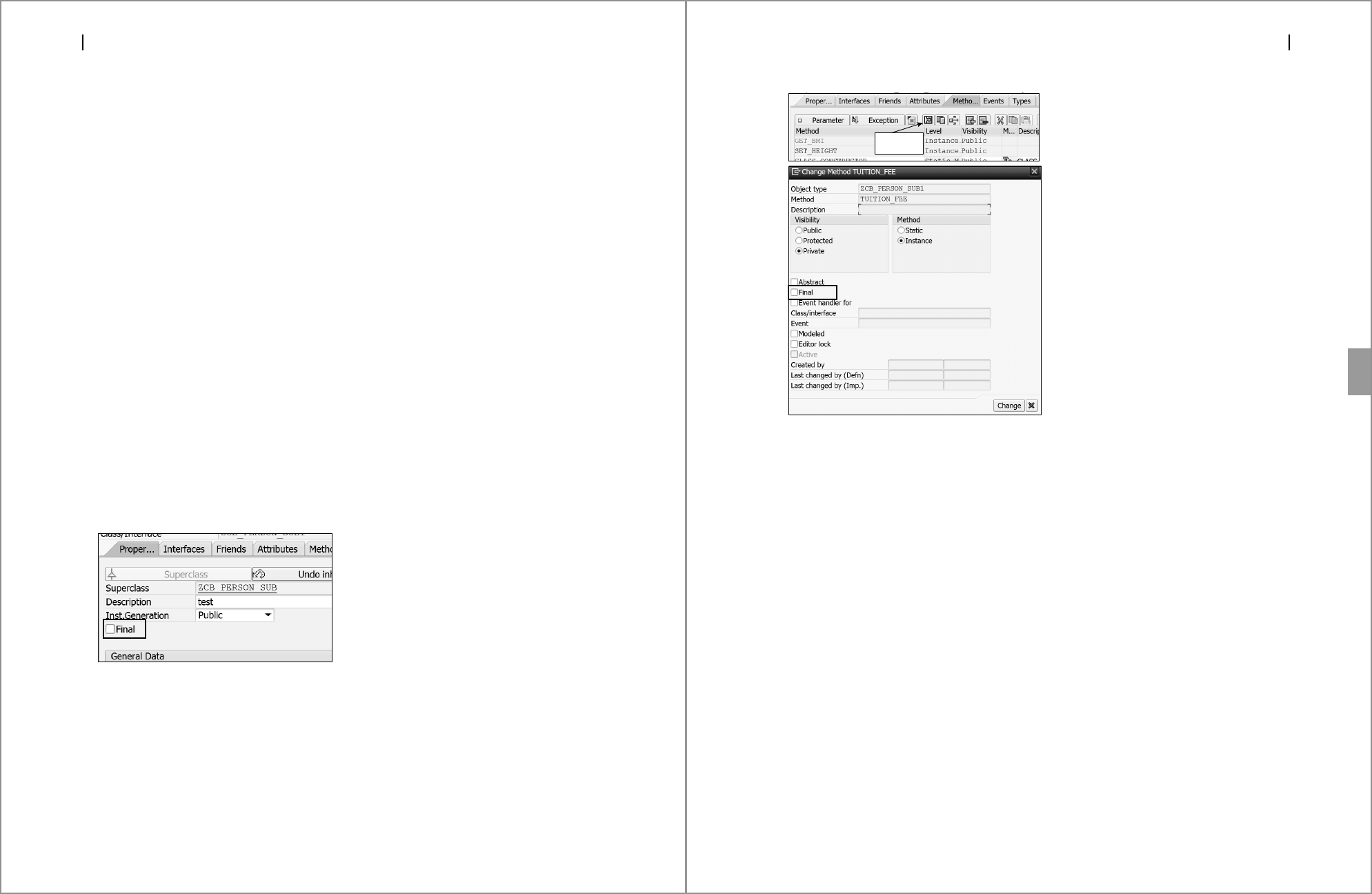
Object-Oriented ABAP

344

8.3.3 Final Classes and Methods

Sometimes, in the inheritance tree, it may not make sense to expand a class fur-

ther. In such a scenario, you can make the class final, which means it can’t be

inherited further. A local class can be defined as a final class by adding

FINAL to

the

CLASS DEFINITION statement, as shown in Listing 8.21.

CLASS cl_final DEFINITION FINAL.

……

ENDCLASS.

Listing 8.21 Defining Final Class

For global classes, to define a class as final in Class Builder, the Final checkbox

needs to be selected in the Properties tab, as shown in Figure 8.8.

Methods can also be defined as final so that they can’t be redefined further in the

subclass. For example, it may make sense to further inherit a class, but a method

in the class may not need to be extended further because it’s purpose is complete.

You can make a method final by adding

FINAL to the METHODS statement, as shown

in Listing 8.22.

CLASS cl_parent DEFINITION.

PUBLIC SECTION.

METHODS student FINAL.

ENDCLASS.

Listing 8.22 Final Method

Figure 8.8 Final Class

To make the method of a global class final, keep the cursor on the method in the

Class Builder and select the Detail View button. In the Change Method window,

select the Final checkbox, as shown in Figure 8.9.

Inheritance

8.3

345

Figure 8.9 Final Method in Class Builder

8.3.4 Composition

Using inheritance, we design classes that fit an is a relationship. For example, a

commerce student is a type of student, so we define the class

commerce_student

as a subclass of student in the example in Listing 8.20. Sometimes, in an effort to

reuse the existing code, developers create an inheritance tree that doesn’t fit an is

a relationship. For example, if we have an existing

orders class, it makes sense to

create a

sales_order class inheriting from the orders class, because a sales order

is an order.

However, if you want to define a class for

delivery, it may not make sense to

inherit the

orders class, because a delivery is not an order. However, each order

has one or more deliveries associated with it. If the objects fit the has a relation-

ship, we call it a composition relationship.

Composition allows you to reuse existing functionality by maintaining the exist-

ing object as an attribute in the class. Therefore, the

orders class can have deliv-

ery

as an attribute in the class. This arrangement allows you to take advantage of

the existing functionality in the system, as shown in Listing 8.23.

Detail View

button

Object-Oriented ABAP

346

CLASS cl_delivery DEFINITION.

PUBLIC SECTION.

METHODS get_delivery.

ENDCLASS.

CLASS cl_delivery IMPLEMENTATION.

METHOD get_delivery.

ENDMETHOD.

ENDCLASS.

CLASS cl_orders DEFINITION.

PUBLIC SECTION.

METHODS track_order.

PRIVATE SECTION.

DATA delivery TYPE REF TO cl_delivery.

ENDCLASS.

CLASS cl_orders IMPLEMENTATION.

METHOD track_order.

CREATE OBJECT delivery.

delivery->get_delivery( ).

ENDMETHOD.

ENDCLASS.

Listing 8.23 Composition Example

In Listing 8.23, the cl_delivery class is maintained as an attribute in the cl_

orders

class. The delivery object is instantiated in the track method to access the

delivery information about the order.

Tip

As a rule of thumb, use an inheritance relationship between objects if they fit the is a

relationship and use composition if the objects fit the has a relationship. This tip should

help you make better design decisions.

8.3.5 Refactoring Assistant

When you’re designing an application, sometimes you may miss defining the

class components at the right level in the inheritance hierarchy. For example, you

may have defined a method in the subclass that may make more sense in the

superclass due to a change in the requirement.

In such a scenario, you can use the refactoring assistant tool in Class Builder to

move the class components up or down the inheritance tree. This saves a lot of

effort and any chance of missing steps when manually moving the components.

Polymorphism

8.4

347

To use the refactoring assistant, select the menu path Utilities 폷 Refactoring 폷

Refactoring in Class Builder, as shown in Figure 8.10.

Figure 8.10 Refactoring Assistant Menu Path

In the Refactoring Assistant window (see Figure 8.11), you can drag and drop

components to the right hierarchy level.

Figure 8.11 Refactoring Assistant Window

Now that we’ve walked through the inheritance principles, let’s move on to using

polymorphism in OOP.

8.4 Polymorphism

Polymorphism means having many forms. The inheritance concept leads to many

interesting scenarios in which objects can take different forms. For example, it’s

possible for a subclass to respond to a method call of the superclass.

Object-Oriented ABAP

348

To understand polymorphism, you first need to understand static and dynamic

types. We’ll then look at how to use casting when a static type source reference

object isn’t the same as the target reference object. From there, we’ll discuss how

to use dynamic binding with the

CALL method before finally looking at imple-

menting multiple inheritances using interfaces.

8.4.1 Static and Dynamic Types

The static type of an object (reference variable) is the class type that is used to

define an object. For example, in Listing 8.24, the

oref reference is defined by

referring to the

cl_class class. In this case, the static type of the oref object is the

cl_class class as it’s statically defined in the code.

CLASS cl_class DEFINITION.

PUBLIC SECTION.

METHODS meth.

ENDCLASS.

CLASS cl_class IMPLEMENTATION.

METHOD meth.

ENDMETHOD.

ENDCLASS.

DATA oref TYPE REF TO cl_class.

Listing 8.24 Code Defining Reference Object

Sometimes, you may want to assign one reference object to another reference

object that doesn’t share the same static type. For example, because instances of

classes in an inheritance tree are interchangeable, you can assign the instance of

the subclass to the instance of the superclass, as shown in Listing 8.25, by using

the

parent = child statement.

CLASS cl_parent DEFINITION.

PUBLIC SECTION.

METHODS meth1.

METHODS meth2.

ENDCLASS.

CLASS cl_parent IMPLEMENTATION.

METHOD meth1.

WRITE 'In method1 of parent'.

ENDMETHOD.

METHOD meth2.

WRITE 'In method2 of parent'.

ENDMETHOD.

ENDCLASS.

Polymorphism

8.4

349

CLASS cl_child DEFINITION INHERITING FROM cl_parent.

PUBLIC SECTION.

METHODS meth2 REDEFINITION.

METHODS meth3.

ENDCLASS.

CLASS cl_child IMPLEMENTATION.

METHOD meth2.

WRITE 'In method2 of child'.

ENDMETHOD.

METHOD meth3.

WRITE 'In method3 of child'.

ENDMETHOD.

ENDCLASS.

DATA parent TYPE REF TO cl_parent.

DATA child TYPE REF TO cl_child.

START-OF-SELECTION.

CREATE OBJECT parent.

CREATE OBJECT child.

Parent->meth2( ).

parent = child.

parent->meth2( ).

Listing 8.25 Example of Casting

In Listing 8.25, once the reference object parent is instantiated using the CREATE

OBJECT

statement, it sets the pointer (in memory) of the parent reference object

to the

cl_parent class. The pointer to which the reference object points at run-

time is called the dynamic type of the object.

At this point, both the static type and dynamic type of the

parent object are the

same. The

parent = child statement assigns the instance of the child object to the

parent object. When one reference object is assigned to another reference object,

the object itself is not assigned; only the pointer of the object is moved. In other

words, after the assignment

parent = child, the parent object points to the mem-

ory location of the

child object. After this assignment, the dynamic type of the

parent object is changed to the cl_child class and the static type is cl_parent.

At this point in the code, both the

parent and child reference objects are point-

ing to the same

cl_child object. Because there’s no reference to the parent object

after this assignment, the

parent object will be removed from the memory auto-

matically by the garbage collector. The ABAP runtime environment calls the gar-

bage collector periodically to remove objects from memory that are no longer ref-

erenced by object reference variables.

Object-Oriented ABAP

350

In Listing 8.25, when the parent->meth2( ) method is first called before the par-

ent

= child assignment (that is, before its dynamic type is changed), it will exe-

cute the code in the

meth2 method of the cl_parent superclass. However, the

same statement after the

parent = child assignment will execute the code in the

meth2 method of the cl_child subclass, effectively displaying polymorphism

because the same object behaves differently during the runtime of the program.

8.4.2 Casting

Similar to the conversion rules applied when different types of data objects are

assigned to each other, the assignment of objects of different static types are gov-

erned by certain rules. If the static type of the source reference object is not the

same as the target reference object, then a special operation called a cast must

occur. This process is known as casting. For the cast operation to work, the static

type of the target reference object should be same or more general than the

dynamic type of the source reference object.

In the example in Listing 8.25, the

cl_parent parent object is more generic than

the

cl_child child object (a superclass will always be the same as or more generic

than a subclass). In other words, the parent class has implemented two methods,

whereas the subclass has become more specific by implementing a third method

not available in the parent class. Therefore, the parent class is more generic than

the child class, and for this reason, we could assign the child object to the parent

object.

There are two different types of cast operations possible: a narrowing cast (or up

cast) and a widening cast (or down cast). The following subsections look at these

different casting operations.

Narrowing Cast

A narrowing cast occurs when the static type of the target reference object is

more generic than the static type of the source reference object. The casting oper-

ation we performed in Listing 8.25 is a narrowing cast. It’s called a narrowing cast

because the parent class is more generic, and after casting the parent class can

only access the components of the child class that are defined in the static type of

the parent class, effectively reducing the scope of (narrowing) the components

that can be accessed.

Polymorphism

8.4

351

For example, say a parent class has two methods, meth1 and meth2, and the child

class has an additional method,

meth3, which isn’t defined in the parent class.

After the casting operation, you can only access the

meth1 and meth2 methods of

the child class by using the parent object reference. If you try to access the

meth3

method, it will result in a syntax error, as shown in Listing 8.26. You can, how-

ever, access the

meth3 method using the child object reference, because it still

exists in the program and isn’t truncated.

Parent = child. "Assigns child reference to parent.

Parent->meth1( )."Calls the method meth1 in child if redefined.

Parent->meth2( )."Calls the method meth2 in child if redefined.

Parent->meth3( )."Results in syntax error.

Child->meth3( )."Works as expected.

Listing 8.26 Narrow Cast

The narrow cast can also be performed during instantiation by adding TYPE to the

CREATE OBJECT statement as shown:

DATA parent TYPE REF TO cl_parent.

CREATE OBJECT parent TYPE cl_child.

Widening Cast

A widening cast occurs when the static type of the target reference object is more

specific than the static type of the source reference object. Because this contra-

venes the rule for casting, which specifies that the target object should always be

more generic than the source object, the syntax checker will complain that the

source object can’t be converted to the target object if you try to assign the

objects using the

= operator or use the MOVE statement. To bypass this restriction

and tell the compiler that we know what we’re doing, we use the

?= operator for

a widening cast, as shown:

Child ?= parent.

Using the ?= operator will only bypass the check statically during compile time

and postpones it until runtime. It will throw a runtime error if the target object is

not more generic than the source object.

For example, the code in Listing 8.27 will pass the syntax checker (static check)

but result in a runtime error because the child object is more specific than the par-

ent object.

Object-Oriented ABAP

352

CLASS cl_parent DEFINITION.

PUBLIC SECTION.

METHODS meth1.

METHODS meth2.

ENDCLASS.

CLASS cl_parent IMPLEMENTATION.

METHOD meth1.

WRITE 'In method1 of parent'.

ENDMETHOD.

METHOD meth2.

WRITE 'In method2 of parent'.

ENDMETHOD.

ENDCLASS.

CLASS cl_child DEFINITION INHERITING FROM cl_parent.

PUBLIC SECTION.

METHODS meth2 REDEFINITION.

METHODS meth3.

ENDCLASS.

CLASS cl_child IMPLEMENTATION.

METHOD meth2.

WRITE 'In method2 of child'.

ENDMETHOD.

METHOD meth3.

WRITE 'In method3 of child'.

ENDMETHOD.

ENDCLASS.

DATA parent TYPE REF TO cl_parent.

DATA child TYPE REF TO cl_child.

START-OF-SELECTION.

CREATE OBJECT parent.

CREATE OBJECT child.

Child ?= parent. "Results in runtime error

Listing 8.27 Widening Cast Resulting in Runtime Error

A widening cast should only be used when the dynamic type of the target object

will be generic than the source object. This effectively means that a narrowing

cast must be performed before a widening cast, as shown in Listing 8.28. Widen-

ing casts can be confusing and dangerous, so they should be used with care.

CLASS cl_parent DEFINITION.

PUBLIC SECTION.

METHODS meth1.

METHODS meth2.

ENDCLASS.

CLASS cl_parent IMPLEMENTATION.

METHOD meth1.

WRITE 'In method1 of parent'.

ENDMETHOD.

Polymorphism

8.4

353

METHOD meth2.

WRITE 'In method2 of parent'.

ENDMETHOD.

ENDCLASS.

CLASS cl_child1 DEFINITION INHERITING FROM cl_parent.

PUBLIC SECTION.

METHODS meth2 REDEFINITION.

METHODS meth3.

ENDCLASS.

CLASS cl_child1 IMPLEMENTATION.

METHOD meth2.

WRITE 'In method2 of child1'.

ENDMETHOD.

METHOD meth3.

WRITE 'In method3 of child1'.

ENDMETHOD.

ENDCLASS.

CLASS cl_child2 DEFINITION INHERITING FROM cl_child1.

PUBLIC SECTION.

METHODS meth2 REDEFINITION.

METHODS meth3 REDEFINITION.

METHODS meth4.

ENDCLASS.

CLASS cl_child2 IMPLEMENTATION.

METHOD meth2.

WRITE 'In method2 of child2'.

ENDMETHOD.

METHOD meth3.

WRITE 'In method3 of child2'.

ENDMETHOD.

METHOD meth4.

WRITE 'In method4 of child2'.

ENDMETHOD.

ENDCLASS.

DATA parent TYPE REF TO cl_parent.

DATA child1 TYPE REF TO cl_child1.

DATA child2 TYPE REF TO cl_child2.

START-OF-SELECTION.

CREATE OBJECT parent.

CREATE OBJECT child1.

CREATE OBJECT child2.

parent = child2.

child1 ?= parent.

child1->meth2( ).

Listing 8.28 Widening Cast Example

Object-Oriented ABAP

354

In Listing 8.28, three classes are defined: cl_parent, cl_child1, and cl_child2.

cl_child1 inherits from cl_parent, and Cl_child2 inherits from cl_child1.

A narrow cast is first performed by assigning the

child2 object to the parent

object, and then a widening cast is performed by assigning the parent object to

child1. When the meth2 method is called using the child1 object reference after

the widening cast, it will execute the code in the

meth2 method of the cl_child2

class.

8.4.3 Dynamic Binding with the CALL Method

When an object is passed to the method as a parameter, the system automatically

binds the object dynamically. This allows us to design objects that are easily

extendable.

To understand dynamic binding with the

CALL method, let’s look at the code snip-

pet in Listing 8.29. Here, we’ve defined

cl_student as an abstract class with

tuition_fee and get_fee as abstract methods with public visibility. A fee_paid

attribute that can be set if the fee is paid by the student is defined in the protected

section.

Two classes,

cl_commerce_student and cl_science_student, inherit the cl_stu-

dent

class and maintain their own implementation of the tuition_fee and get_

fee

abstract methods. In the tuition_fee method, the private fee_paid attribute

is set to

abap_true if the student has paid the fee. The get_fee method returns the

value of the private

fee_paid attribute.

We’ve defined one

cl_admission class that can be used to enroll a student in a

course. This class has two methods,

set_student and enroll, which can be used

to complete the admission of the student in a course. Because this

cl_admission

class should be able to enroll any student from any student category (science stu-

dent, commerce student, etc.), we need to design this class to import information

about any student category.

The

set_student method of the cl_admission class is defined with an importing

parameter to import the

student object. If we maintain the static type of this

importing parameter as

cl_commerce_student, it can only import the commerce

student object and our class can only process the admission for commerce stu-

dents. Similarly, if we maintain the static type of the importing parameter as

cl_

science_student

, it can only import the science student object and our class can

Polymorphism

8.4

355

only process the admission for science students. In order to make it work for any

student category, we’ve maintained the importing parameter of this method as a

static type of the

cl_student abstract class, from which the cl_science_student

and cl_commerce_student classes inherit.

CLASS cl_student DEFINITION ABSTRACT.

PUBLIC SECTION.

METHODS tuition_fee ABSTRACT.

METHODS get_fee ABSTRACT RETURNING VALUE(fee_paid) TYPE boolean.

PROTECTED SECTION.

DATA fee_paid TYPE boolean.

ENDCLASS.

CLASS cl_commerce_student DEFINITION INHERITING FROM cl_student.

PUBLIC SECTION.

METHODS tuition_fee REDEFINITION.

METHODS get_fee REDEFINITION.

ENDCLASS.

CLASS cl_commerce_student IMPLEMENTATION.

METHOD tuition_fee.

"logic to calculate tuition fee for commerce students goes here

"IF fee paid.

fee_paid = abap_true.

ENDMETHOD.

METHOD get_fee.

fee_paid = me->fee_paid.

ENDMETHOD.

ENDCLASS.

CLASS cl_science_student DEFINITION INHERITING FROM cl_student.

PUBLIC SECTION.

METHODS tuition_fee REDEFINITION.

METHODS get_fee REDEFINITION.

ENDCLASS.

CLASS cl_science_student IMPLEMENTATION.

METHOD tuition_fee.

"logic to calculate tuition fee for science students goes here

"IF fee paid.

fee_paid = abap_true.

ENDMETHOD.

METHOD get_fee.

fee_paid = me->fee_paid.

ENDMETHOD.

ENDCLASS.

CLASS cl_admission DEFINITION.

PUBLIC SECTION.

METHODS set_student IMPORTING im_student TYPE REF TO cl_student.

METHODS enroll.

PRIVATE SECTION.

DATA admit TYPE boolean.

ENDCLASS.

Object-Oriented ABAP

356

CLASS cl_admission IMPLEMENTATION.

METHOD set_student.

IF im_student->get_fee( ) EQ abap_true.

admit = abap_true.

ENDIF.

ENDMETHOD.

METHOD enroll.

IF admit EQ abap_true.

*Perform the steps to enroll

ENDIF.

ENDMETHOD.

ENDCLASS.

DATA : commerce_student TYPE REF TO cl_commerce_student,

science_student TYPE REF TO cl_science_student,

admission TYPE REF TO cl_admission.

START-OF-SELECTION.

CREATE OBJECT: commerce_student,

science_student,

admission.

CALL METHOD commerce_student->tuition_fee.

CALL METHOD admission->set_student( EXPORTING im_student = commerce_

student ).

CALL METHOD admission->enroll.

CALL METHOD science_student->tuition_fee.

CALL METHOD admission->set_student( EXPORTING im_student = science_

student ).

CALL METHOD admission->enroll.

Listing 8.29 Code for Dynamic Call Method Binding

When the set_student method of the cl_admission class is called, it allows us to

pass any student object that is inherited from

cl_student. Within this method,

we’re checking if the student has paid the fee by calling the

get_fee method of

the imported object and accordingly processing the admission of the student.

Here, even though the static type of the imported object is different from the

static type of the importing parameter, the system automatically binds the object

to the correct instance.

With this design, we can easily process admissions for any future student cate-

gory via the

cl_admission class. All the student category class needs to do is to

inherit the abstract class

cl_student.

Polymorphism

8.4

357

8.4.4 Interfaces

Similar to Java, ABAP Objects only supports single inheritance and don’t support

multiple inheritance as in C++. Single inheritance means a class can have multiple

subclasses but only one superclass. Many subclasses can use the same class as

their superclass, but each subclass can only have a single superclass.

Modern programming languages didn’t add support for multiple inheritance

(having multiple superclasses) in order to avoid ambiguity. One of the common

problems with multiple inheritance is called the diamond problem. For example,

as depicted in Figure 8.12, assume you have two subclasses

B and C inheriting

from the same superclass

A and that both classes B and C have redefined a method

XYZ of class A in their implementation. Now, if a new subclass D is defined as hav-

ing both class

B and class C as its superclasses then which superclass method will

it use?

Figure 8.12 Diamond Problem with Multiple Inheritance

One way of implementing multiple inheritance is to use interfaces. Interfaces pro-

vide all the advantages of multiple inheritance while avoiding all the problems.

Interfaces are defined similarly to classes via the

INTERFACE statement. An inter-

face only contains a definition for which the implementation is maintained in the

class that uses the interface. If you need a common definition in multiple classes,

then you can create an interface and use it in multiple classes.

Class A

Method xyz

Class C INHERITING FROM A

Class B INHERITING FROM A

Methods xyz REDEFINITION

Class D INHERITING FROM A B

Methods xyz REDEFINITION

Methods xyz

Which implementation is

called? Class B or Class C?

Object-Oriented ABAP

358

The syntax to define an interface is shown in Listing 8.30, in which interface if_

student

is defined using the INTERFACE statement and ended with the ENDINTER-

FACE

statement.

INTERFACE if_student.

DATA course TYPE char10.

METHODS meth1.

EVENTS enrolled.

ENDINTERFACE.

CLASS cl_science DEFINITION.

PUBLIC SECTION.

INTERFACES if_student.

ENDCLASS.

CLASS cl_science IMPLEMENTATION.

METHOD if_student~meth1.

ENDMETHOD.

ENDCLASS.

Listing 8.30 Interfaces

An interface can have all the components that a class supports, such as methods,

attributes, events, and so on. All of the components are in

PUBLIC SECTION by

default, and you can’t use any visibility section in the interface definition.

Because an interface is generally created to be used in multiple classes, it makes

sense to use the interface to define the public interface of the class, with each class

that uses the interface implementing its own private or protected components.

In Listing 8.30, a

cl_science class implements the if_student interface via the

INTERFACES statement. In the implementation of the cl_science class, the meth1

method defined in the if_student interface is implemented. Because the meth1

method is defined in the interface and not in the class itself, the method is

accessed using the

interface_name~component_name syntax. Here, the tilde sym-

bol (

~) is the interface component selector that should be used to access the com-

ponent of an interface.

Unlike classes, interfaces do not have any implementation section. Interfaces can

be defined only in the global declaration area of a program and can’t be defined

within a class or a procedure or an event block.

Sometimes, the interface name can be too long. To avoid addressing the interface

component using the long interface name, we can use aliases to make it easy

while coding, as shown in Listing 8.31.

Polymorphism

8.4

359

INTERFACE if_student.

DATA course TYPE char10.

METHODS meth1.

EVENTS enrolled.

ENDINTERFACE.

CLASS cl_science DEFINITION.

PUBLIC SECTION.

INTERFACES if_student.

ALIASES m1 FOR if_student~meth1.

ENDCLASS.

CLASS cl_science IMPLEMENTATION.

METHOD m1.

ENDMETHOD.

ENDCLASS.

DATA science TYPE REF TO cl_science.

START-OF-SELECTION.

CREATE OBJECT science.

science->m1().

Listing 8.31 Using Aliases

Interfaces can be nested by using the INTERFACES statement to include an inter-

face within an interface. In Listing 8.32, the

if_student interface is nested inside

if_college. An alias is defined for the meth1 method of if_student within if_

college

. The cl_science class implements the if_college interface. The meth1

method of the if_student interface is accessed within the class using the alias

defined for it in

if_college.

INTERFACE if_student.

DATA course TYPE char10.

METHODS meth1.

EVENTS enrolled.

ENDINTERFACE.

INTERFACE if_college.

INTERFACES if_student.

ALIASES m1 FOR if_student~meth1.

METHODS meth1.

ENDINTERFACE.

CLASS cl_science DEFINITION.

PUBLIC SECTION.

INTERFACES if_college.

ALIASES m1 FOR if_college~m1.

ALIASES m2 FOR if_college~meth1.

ENDCLASS.

CLASS cl_science IMPLEMENTATION.

METHOD m1.

ENDMETHOD.

Object-Oriented ABAP

360

METHOD m2.

ENDMETHOD.

ENDCLASS.

DATA science TYPE REF TO cl_science.

START-OF-SELECTION.

CREATE OBJECT science.

science->m1( ).

Listing 8.32 Nesting Interfaces

The process of defining a global interface in Class Builder is similar to creating a

class. Follow these steps to create an interface in Class Builder:

1. On the initial Class Builder screen (Transaction SE24; see Figure 8.13), enter the

name of the interface and click the Create button. If the name starts with ZIF,

Class Builder will automatically create an interface; otherwise, you’ll see a

dialog box (see Figure 8.14) to choose whether to create a class or interface.

Figure 8.13 Class Builder: Initial Screen

Figure 8.14 Object Type Selection Dialog Box

2. On the Class Builder: Change Interface… screen (see Figure 8.15), maintain

the components of the interface and click the Activate button in the applica-

tion toolbar to activate.

Polymorphism

8.4

361

Figure 8.15 Class Builder: Change Interface Screen

3. You can include the interface in a global class under the Interfaces tab, as

shown in Figure 8.16.

Figure 8.16 Including Interface in Global Class

4. The alias for an interface component can be maintained under the Aliases tab,

as shown in Figure 8.17. The name of the alias is maintained under the Alias

column, and the visibility for the alias can be set under the Visible column.

Figure 8.17 Aliases for Interface Component

Object-Oriented ABAP

362

In this section, we discussed the concept of polymorphism in OOP. In the next

section, we’ll take a bit of a departure from object-oriented concepts and look at

how to work with XML.

8.5 Working with XML

Extensible Markup Language (XML) is a meta markup language that is used to

define structured documents that can be easily exchanged between heteroge-

neous systems. There are many ways to exchange data between systems, but with

the growth of web services, XML has gained popularity among developers. The

beauty of XML lies in its flexibility and simplicity.

XML defines a standard that can be used to define the format of documents.

Using XML, we can structure and organize various kind of data. A markup lan-

guage (e.g., HTML) consists of tags, which are predefined. Tags allow you to for-

mat and organize the data. Tags are maintained between less than (

<) and greater

than (

>) symbols. For example, in an HTML document, we can open the para-

graph tag with

<p> and close it with </p>. The content maintained between the

tags is interpreted accordingly. Here, the content maintained between

<p> and </

is formatted as a paragraph; the content maintained between <h1> and </h1> is

interpreted as a header.

However, XML is a meta markup language, which defines a markup language. It’s

designed to be flexible and easy to understand for both humans and machines. In

XML, there are no predefined tags; any tag can be used to describe content.

Even though an in-depth understanding of XML documents and their processing

is beyond the scope of this book, in this section we’ll discuss the basic XML syn-

tax and look at the iXML library provided by SAP to create XML documents in

ABAP. Understanding XML is helpful when exposing or consuming data with

external applications. This section should help you appreciate how OOP aids in

designing libraries that are easy for developers to use in their programs.

8.5.1 XML Overview

XML files provide great flexibility to share structured documents. Because there

are no predefined tags, we can use tags that suit our domain and that are self-

Working with XML

8.5

363

explanatory. Of course, developing a standard for document markup makes it

easy for third-party vendors to develop software that can process XML files.

For example, say we have a website that can be extended by installing custom

extensions. The extensions are of two types: components and plugins (i.e., the

website can be extended by developing a component or a plugin). We’ve devel-

oped a component and want to upload the files of the custom component as a

package to the webserver. To provide the information about the component to

the installer script, we can supply an XML file with the package that contains

information about the file structure of the package, as shown in Listing 8.33. The

installer can read this XML file and upload the files in the package to the desig-

nated folders in the web server.

<?xml version="1.0" encoding="utf-8"?>

<!—This is comment-->

<filename>index.html</filename>

</files>

<folder>images</folder>

</media>

</extension>

Listing 8.33 Sample XML Document

As shown in Listing 8.33, XML documents are organized into a series of elements.

The first line in the document specifies the XML version and the encoding used.

The syntax for this statement is

<?xml version="1.0" encoding=""?> and it’s

optional.

The basic syntax to define an element in XML is as follows:

<element_name attribute_name=attribute_value>

</element_name>

In the example XML file provided, for the <extension type="component"> tag, the

element name is

extension, the attribute name is type, and the attribute value is

component. This tells the upload script that we’re trying to upload an extension

that’s a component. The tags

<files> and <media> are the elements under the

Object-Oriented ABAP

364

parent node <extension>. The tags under <files> and <media> are the respective

elements’ content, which specifies the folders and files that we are uploading. The

document is closed with the closing tag

</extension>. Comments can be main-

tained between

.

XML markup is case-sensitive; for example, the element name

<ELEMENT> is differ-

ent than

<element>.

8.5.2 XML Processing Concepts

SAP NetWeaver AS ABAP provides an iXML library that can be used to process

XML files. This library implements various interfaces that allow us to work with

XML files by calling various methods.

Listing 8.34 shows the code to create an XML file using the iXML library. The

XML file we’re creating contains the data from Listing 8.33. In Listing 8.34, we’re

defining reference objects for the XML document from the iXML library. The

reference object for the XML document is referenced to the

if_ixml_document

interface, and a reference object is defined for each element in the XML file by

referencing

if_ixml_element. The XML file is generated by calling the respective

methods from the library, as shown in Listing 8.34.

REPORT ZDEMO_XML.

*Declarations to create XML document

DATA: lr_ixml TYPE REF TO if_ixml. "Reference for iXML object

"Reference for XML document

DATA: lr_document TYPE REF TO if_ixml_document.

."Reference for "extension" element in document

DATA: lr_extension TYPE REF TO if_ixml_element

."Reference for "files" element in document

DATA: lr_files TYPE REF TO if_ixml_element

."Reference for "media" element in document

DATA: lr_media TYPE REF TO if_ixml_element

."Reference to set encoding

DATA: lr_encoding TYPE REF TO if_ixml_encoding

*Declarations to create output stream and render the file to

*application server directory

DATA: lr_streamfactory TYPE REF TO if_ixml_stream_factory,

lr_ostream TYPE REF TO if_ixml_ostream,

lr_renderer TYPE REF TO if_ixml_renderer.

DATA file_path TYPE string VALUE 'D:\USR\SAP\PUT\MANIFEST.XML'.

Working with XML

8.5

365

* Create iXML object

lr_ixml = cl_ixml=>create( ).

*Create Document

lr_document = lr_ixml->create_document( ).

*Create encoding

lr_encoding = lr_ixml->create_encoding( BYTE_ORDER = 0 CHARACTER_SET =

'UTF-8').

*Set encoding

lr_document->set_encoding( lr_encoding ).

*Create element "extension" as root

lr_extension = lr_document->create_simple_element(

name = 'extension'

parent = lr_document ).

*Set attribute for the "extension" element

lr_extension->set_attribute( name = 'Type'

VALUE = 'Component' ).

*Create "files" element with "extension" element as parent

lr_files = lr_document->create_simple_element(

name = 'files'

parent = lr_extension ).

*Set attribute for "files" element

lr_files->set_attribute( name = 'Folder'

VALUE = 'site' ).

*Create element content

lr_document->create_simple_element( name = 'filename'

parent = lr_files

VALUE = 'index.html' ).

lr_document->create_simple_element( name = 'filename'

parent = lr_files

VALUE = 'site.php' ).

*Create "media" element with "extension" element as parent

lr_media = lr_document->create_simple_element(

name = 'media'

parent = lr_extension ).

**Set attribute for "media" element

lr_media->set_attribute( name = 'Folder'

VALUE = 'media' ).

*Create element content

lr_document->create_simple_element( name = 'folder'

parent = lr_media

VALUE = 'css' ).

lr_document->create_simple_element( name = 'folder'

parent = lr_media

VALUE = 'images' ).

lr_document->create_simple_element( name = 'folder'

parent = lr_media

VALUE = 'js' ).

Object-Oriented ABAP

366

* Create stream factory

lr_streamfactory = lr_ixml->create_stream_factory( ).

* Create output stream

lr_ostream = lr_streamfactory->create_ostream_uri( system_id = file_

path ).

* Create renderer

lr_renderer = lr_ixml->create_renderer( ostream = lr_ostream

document = lr_document ).

* Set pretty print

lr_ostream->set_pretty_print( abap_true ).

* Renders the attached document into output stream

lr_renderer->render( ).

Listing 8.34 Using iXML library to Create XML File

The code in Listing 8.34 saves the XML file in the application server directory, as

shown in Figure 8.18.

Figure 8.18 XML File

8.6 Summary

In this chapter, we explored various OOP concepts. The four pillars of OOP are

encapsulation, inheritance, polymorphism, and abstraction. We discussed all of

these concepts and looked at the various ways they’re implemented in ABAP.

Summary

8.6

367

By now, you should have a good overview of objects and should feel comfortable

working with ABAP Objects. Designing software using ABAP Objects takes some

experience, but this chapter should serve as a starting point for you to start look-

ing at designing applications by using OOP concepts.

In the next chapter, we’ll use some of the concepts from this chapter to shed light

on how to handle error situations in applications.

Contents

Acknowledgments ............................................................................................ 21

Preface ............................................................................................................. 23

1 Introduction to ERP and SAP ................................................... 29

1.1 Historical Overview ...................................................................... 29

1.2 Understanding an ERP System ...................................................... 32

1.2.1 What Is ERP? ................................................................... 32

1.2.2 ERP vs. Non-ERP Systems ................................................ 33

1.2.3 Advantages of an ERP System .......................................... 35

1.3 Introduction to SAP ...................................................................... 36

1.3.1 Modules in SAP ............................................................... 36

1.3.2 Types of Users ................................................................. 37

1.3.3 Role of an ABAP Consultant ............................................ 38

1.3.4 Changing and Adapting the Data Structure ...................... 40

1.4 ABAP Overview ............................................................................ 43

1.4.1 Types of Applications ...................................................... 43

1.4.2 RICEF Overview .............................................................. 43

1.5 System Requirements ................................................................... 48

1.6 Summary ...................................................................................... 48

2 Architecture of an SAP System ................................................ 49

2.1 Introduction to the Three-Tier Architecture .................................. 49

2.2 SAP Implementation Overview ..................................................... 52

2.2.1 SAP GUI: Presentation Layer ........................................... 52

2.2.2 Application Servers and Message Servers:

Application Layer ............................................................ 54

2.2.3 Database Server/RDBMS: Database Layer ........................ 61

2.3 Data Structures ............................................................................. 64

2.3.1 Client Overview .............................................................. 64

2.3.2 Client-Specific and Cross-Client Data ............................... 65

2.3.3 Repository ....................................................................... 68

2.3.4 Packages ......................................................................... 68

2.3.5 Transport Organizer ........................................................ 70

2.4 Summary ...................................................................................... 75

Contents

3 Introduction to the ABAP Environment ................................... 77

3.1 SAP Environment ......................................................................... 78

3.1.1 ABAP Programming Environment ................................... 78

3.1.2 Logging On to the SAP Environment .............................. 78

3.1.3 Elements of the SAP Screen ............................................ 79

3.1.4 Transaction Codes .......................................................... 82

3.1.5 Navigating and Opening Transactions ............................. 83

3.2 ABAP Workbench Overview ........................................................ 87

3.2.1 ABAP Editor ................................................................... 88

3.2.2 Function Builder ............................................................. 90

3.2.3 Class Builder ................................................................... 91

3.2.4 Screen Painter ................................................................ 92

3.2.5 Menu Painter ................................................................. 95

3.2.6 ABAP Data Dictionary .................................................... 96

3.2.7 Object Navigator ............................................................ 98

3.3 Eclipse IDE Overview ................................................................... 99

3.4 Summary ..................................................................................... 105

4 ABAP Programming Concepts .................................................. 107

4.1 General Program Structure .......................................................... 108

4.1.1 Global Declarations ........................................................ 108

4.1.2 Procedural ..................................................................... 109

4.2 ABAP Syntax ................................................................................ 110

4.2.1 Basic Syntax Rules .......................................................... 110

4.2.2 Chained Statements ....................................................... 111

4.2.3 Comment Lines .............................................................. 112

4.3 ABAP Keywords .......................................................................... 113

4.4 Introduction to the TYPE Concept ............................................... 114

4.4.1 Data Types ..................................................................... 115

4.4.2 Data Elements ................................................................ 130

4.4.3 Domains ........................................................................ 134

4.4.4 Data Objects .................................................................. 137

4.5 ABAP Statements ........................................................................ 141

4.6 Creating Your First ABAP Program ............................................... 143

4.7 Summary ..................................................................................... 149

Contents

5 Structures and Internal Tables ................................................. 151

5.1 Defining Structures ....................................................................... 152

5.1.1 When to Define Structures .............................................. 154

5.1.2 Local Structures ............................................................... 155

5.1.3 Global Structures ............................................................. 158

5.1.4 Working with Structures .................................................. 162

5.1.5 Use Cases ........................................................................ 163

5.2 Internal Tables .............................................................................. 164

5.2.1 Defining Internal Tables .................................................. 164

5.2.2 Types of Internal Tables ................................................... 167

5.2.3 Table Keys ....................................................................... 171

5.2.4 Working with Internal Tables .......................................... 175

5.2.5 Control Break Statements ................................................ 182

5.3 Introduction to Open SQL Statements .......................................... 187

5.3.1 Database Overview ......................................................... 189

5.3.2 Selecting Data from Database Tables ............................... 198

5.3.3 Selecting Data from Multiple Tables ................................ 200

5.4 Processing Data from Database via Internal Tables and

Structures ..................................................................................... 203

5.5 Introduction to the Debugger ....................................................... 205

5.6 Practice ........................................................................................ 209

5.7 Summary ...................................................................................... 209

6 User Interaction ....................................................................... 211

6.1 Selection Screen Overview ........................................................... 212

6.1.1 PARAMETERS ................................................................. 214

6.1.2 SELECT-OPTIONS ........................................................... 221

6.1.3 SELECTION-SCREEN ....................................................... 229

6.1.4 Selection Texts ................................................................ 230

6.2 Messages ...................................................................................... 231

6.2.1 Types of Messages ........................................................... 231

6.2.2 Messages Using Text Symbols ......................................... 233

6.2.3 Messages Using Message Classes ..................................... 235

6.2.4 Dynamic Messages .......................................................... 237

6.2.5 Translation ...................................................................... 238

6.3 Summary ...................................................................................... 239

Contents

7 Modularization Techniques ...................................................... 241

7.1 Modularization Overview ............................................................ 242

7.2 Program Structure ....................................................................... 245

7.2.1 Processing Blocks ........................................................... 246

7.2.2 Event Blocks ................................................................... 258

7.2.3 Dialog Modules .............................................................. 260

7.2.4 Procedures ..................................................................... 261

7.3 Events ......................................................................................... 261

7.3.1 Program Constructor Events ........................................... 262

7.3.2 Reporting Events ............................................................ 262

7.3.3 Selection Screen Events .................................................. 269

7.3.4 List Events ...................................................................... 270

7.3.5 Screen Events ................................................................. 271

7.4 Procedures .................................................................................. 272

7.4.1 Subroutines .................................................................... 274

7.4.2 Function Modules .......................................................... 284

7.4.3 Methods ........................................................................ 293

7.5 Inline Declarations ....................................................................... 300

7.5.1 Assigning Values to Data Objects ................................... 301

7.5.2 Using Inline Declarations with Table Work Areas ............ 301

7.5.3 Avoiding Helper Variables .............................................. 302

7.5.4 Declaring Actual Parameters ........................................... 302

7.6 Summary ..................................................................................... 303

8 Object-Oriented ABAP ............................................................. 305

8.1 Introduction to Object-Oriented Programming ............................ 305

8.1.1 Classes ........................................................................... 308

8.1.2 Methods ........................................................................ 313

8.1.3 Instance and Static Components ..................................... 320

8.1.4 Events ............................................................................ 322

8.2 Encapsulation .............................................................................. 325

8.2.1 Component Visibility ...................................................... 326

8.2.2 Friends ........................................................................... 329

8.2.3 Implementation Hiding .................................................. 332

8.3 Inheritance .................................................................................. 335

8.3.1 Inheriting Components ................................................... 336

8.3.2 Abstract Classes and Methods ........................................ 341

8.3.3 Final Classes and Methods ............................................. 344

Contents

8.3.4 Composition ................................................................... 345

8.3.5 Refactoring Assistant ....................................................... 346

8.4 Polymorphism .............................................................................. 347

8.4.1 Static and Dynamic Types ................................................ 348

8.4.2 Casting ............................................................................ 350

8.4.3 Dynamic Binding with the CALL Method ......................... 354

8.4.4 Interfaces ........................................................................ 357

8.5 Working with XML ....................................................................... 362

8.5.1 XML Overview ................................................................ 362

8.5.2 XML Processing Concepts ............................................... 364

8.6 Summary ...................................................................................... 366

9 Exception Handling .................................................................. 369

9.1 Exceptions Overview .................................................................... 369

9.2 Procedural Exception Handling ..................................................... 370

9.2.1 Maintaining Exceptions Using Function Modules ............ 370

9.2.2 Maintaining Exceptions Using Methods ........................... 373

9.2.3 Maintaining Exceptions for Local Classes ......................... 374

9.3 Class-Based Exception Handling ................................................... 375

9.3.1 Raising Exceptions ........................................................... 376

9.3.2 Catchable and Non-Catchable Exceptions ........................ 378

9.3.3 Defining Exception Classes Globally ................................. 383

9.3.4 Defining Exception Classes Locally ................................... 386

9.4 Messages in Exception Classes ...................................................... 387

9.4.1 Using the Online Text Repository .................................... 387

9.4.2 Using Messages from a Message Class ............................. 390

9.4.3 Using the MESSAGE Addition to Raise an Exception ........ 393

9.5 Summary ...................................................................................... 393

10 ABAP Data Dictionary .............................................................. 395

10.1 Database Tables ........................................................................... 396

10.1.1 Creating a Database Table ............................................... 399

10.1.2 Indexes ........................................................................... 409

10.1.3 Table Maintenance Generator ......................................... 414

10.1.4 Foreign Keys ................................................................... 418

10.1.5 Include Structure ............................................................. 422

10.1.6 Append Structure ............................................................ 424

10.2 Views ........................................................................................... 426

10.2.1 Database Views ............................................................... 427

Contents

10.2.2 Projection Views ............................................................ 429

10.2.3 Maintenance Views ........................................................ 431

10.2.4 Help Views ..................................................................... 433

10.2.5 ABAP CDS Views ............................................................ 434

10.3 Data Types .................................................................................. 438

10.3.1 Data Elements ................................................................ 439

10.3.2 Structures ....................................................................... 443

10.3.3 Table Types .................................................................... 446

10.4 Type Groups ................................................................................ 450

10.5 Domains ...................................................................................... 451

10.6 Search Helps ................................................................................ 455

10.6.1 Elementary Search Helps ................................................ 457

10.6.2 Collective Search Helps .................................................. 461

10.6.3 Assigning a Search Help ................................................. 463

10.6.4 Search Help Exits ............................................................ 464

10.7 Lock Objects ............................................................................... 465

10.8 Summary ..................................................................................... 469

11 Persistent Data ........................................................................ 471

11.1 Working with Data in Databases .................................................. 472

11.1.1 Open SQL ...................................................................... 474

11.1.2 Logical Unit of Work ...................................................... 485

11.2 ABAP Object Services .................................................................. 492

11.2.1 Persistence Service Overview ......................................... 493

11.2.2 Building Persistent Classes .............................................. 493

11.2.3 Working with Persistent Objects .................................... 498

11.3 File Interfaces .............................................................................. 498

11.3.1 Working with Files in the Application Server .................. 499

11.3.2 Working with Files in the Presentation Layer .................. 501

11.4 Data Clusters ............................................................................... 503

11.4.1 Exporting Data Clusters to Databases ............................. 505

11.4.2 Importing Data Clusters ................................................. 506

11.5 Security Concepts ........................................................................ 506

11.6 Summary ..................................................................................... 508

12 Dialog Programming ................................................................ 509

12.1 Screen Events .............................................................................. 510

12.2 Screen Elements and Flow Logic .................................................. 513

12.2.1 Components of a Dialog Program ................................... 515

Contents

12.2.2 Screens ........................................................................... 520

12.2.3 Screen Elements .............................................................. 525

12.3 Basic Screen Elements .................................................................. 529

12.3.1 Text Fields ....................................................................... 530

12.3.2 Checkboxes and Radio Buttons ....................................... 531

12.3.3 Push Button .................................................................... 533

12.4 Input/Output Fields ...................................................................... 534

12.5 List Box ........................................................................................ 536

12.6 Table Controls .............................................................................. 537

12.6.1 Create a Table Control without a Wizard ......................... 538

12.6.2 Create a Table Control with a Wizard .............................. 542

12.7 Tabstrip Controls .......................................................................... 544

12.8 Subscreens ................................................................................... 545

12.9 Working with Screens ................................................................... 547

12.9.1 Screen Flow Logic ........................................................... 548

12.9.2 GUI Status ....................................................................... 550

12.9.3 GUI Title ......................................................................... 552

12.9.4 Modifying Screen Fields Dynamically ............................... 553

12.9.5 Field Help and Input Help ............................................... 555

12.9.6 Screen Sequence ............................................................. 556

12.9.7 Assigning Transaction Codes ........................................... 558

12.10 Control Framework ....................................................................... 560

12.10.1 Using Container Controls ................................................. 561

12.10.2 Implementing Custom Controls ....................................... 562

12.11 Practice ........................................................................................ 564

12.11.1 Application Flow ............................................................. 566

12.11.2 Delete Functionality ........................................................ 567

12.11.3 Validations and Autofills ................................................. 567

12.12 Summary ...................................................................................... 568

13 List Screens .............................................................................. 569

13.1 Program Types .............................................................................. 570

13.1.1 Executable Programs ....................................................... 571

13.1.2 Module Pool Programs .................................................... 572

13.1.3 Function Groups ............................................................. 572

13.1.4 Class Pools ...................................................................... 573

13.1.5 Interface Pools ................................................................ 573

13.1.6 Subroutine Pools ............................................................. 573

13.1.7 Type Pools ...................................................................... 574

13.1.8 Include Programs ............................................................ 574

Contents

13.2 Program Execution ...................................................................... 574

13.2.1 Executable Program Flow ............................................... 575

13.2.2 Module Pool Program Flow ............................................ 576

13.2.3 Calling Programs Internally ............................................. 577

13.3 Memory Organization .................................................................. 578

13.4 List Events ................................................................................... 582

13.4.1 TOP-OF-PAGE ............................................................... 583

13.4.2 END-OF-PAGE ............................................................... 585

13.4.3 AT LINE-SELECTION ...................................................... 586

13.4.4 AT USER-COMMAND .................................................... 586

13.5 Basic Lists and Detail Lists ........................................................... 588

13.6 Classical Reports .......................................................................... 592

13.7 Interactive Reports ...................................................................... 592

13.7.1 HIDE .............................................................................. 592

13.7.2 READ LINE ..................................................................... 596

13.7.3 GET CURSOR ................................................................. 597

13.7.4 DESCRIBE LIST ............................................................... 597

13.8 Practice ....................................................................................... 598

13.9 Summary ..................................................................................... 599

14 Selection Screens ..................................................................... 601

14.1 Defining Selection Screens ........................................................... 602

14.2 Selection Screen Events ............................................................... 604

14.3 Input Validations ......................................................................... 606

14.4 Selection Screen Variants ............................................................. 608

14.4.1 Creating a Variant .......................................................... 609

14.4.2 Variant Attributes ........................................................... 613

14.4.3 Table Variables from Table TVARVC ............................... 614

14.4.4 Dynamic Date Calculation .............................................. 616

14.4.5 Dynamic Time Calculation .............................................. 617

14.4.6 User-Specific Variables ................................................... 618

14.5 Executing Programs in the Background ........................................ 619

14.6 Displaying and Hiding Screen Elements Dynamically .................... 621

14.7 Calling Programs via Selection Screens ......................................... 623

14.8 Summary ..................................................................................... 623

15 ALV Reports .............................................................................. 625

15.1 Standard ALV Reports Using the Reuse Library ............................ 626

15.1.1 List and Grid Display: Simple Reports ............................. 627

Contents

15.1.2 Block Display .................................................................. 636

15.1.3 Hierarchical Sequential Display ........................................ 640

15.2 Interactive Reports ....................................................................... 644

15.2.1 Loading a Custom SAP GUI Status ................................... 645

15.2.2 Reacting to User Actions ................................................. 649

15.2.3 Printing TOP-OF-PAGE ................................................... 650

15.3 ALV Reports Using the Control Framework ................................... 650

15.4 ALV Object Model ....................................................................... 653

15.4.1 Table Display .................................................................. 654

15.4.2 Hierarchical Display ......................................................... 655

15.4.3 Tree Object Model .......................................................... 659

15.5 Summary ...................................................................................... 661

16 Dynamic Programming ............................................................. 663

16.1 Field Symbols ............................................................................... 665

16.1.1 Using Field Symbols to Make Programs Dynamic ............. 666

16.1.2 Defining Field Symbols .................................................... 673

16.1.3 Assigning a Data Object .................................................. 674

16.1.4 Checking if a Field Symbol is Assigned ............................. 677

16.1.5 Unassigning a Field Symbol ............................................. 678

16.1.6 Casting ............................................................................ 678

16.2 Data References ........................................................................... 679

16.2.1 Defining Reference Variables ........................................... 680

16.2.2 Getting Data References .................................................. 681

16.2.3 Anonymous Data Objects ................................................ 682

16.2.4 Assignment between Reference Variables ........................ 684

16.3 Runtime Type Services .................................................................. 685

16.3.1 Runtime Type Information .............................................. 686

16.3.2 Runtime Type Creation .................................................... 687

16.4 Dynamic Token Specification ........................................................ 691

16.5 Dynamic Procedure Calls .............................................................. 693

16.6 Dynamic Program Generation ....................................................... 695

16.7 Summary ...................................................................................... 697

17 Debugging ................................................................................ 699

17.1 Classic Debugger .......................................................................... 700

17.1.1 Activating and Using the Classic Debugger ...................... 701

17.1.2 Field View ....................................................................... 705

17.1.3 Table View ...................................................................... 705

Contents

17.1.4 Breakpoints View ........................................................... 706

17.1.5 Watchpoints View .......................................................... 707

17.1.6 Calls View ...................................................................... 708

17.1.7 Overview View ............................................................... 708

17.1.8 Settings View ................................................................. 708

17.1.9 Additional Features ........................................................ 710

17.2 New Debugger ............................................................................ 714

17.2.1 UI and Tools ................................................................... 714

17.2.2 Layout and Sessions ....................................................... 717

17.3 AMDP Debugger ......................................................................... 718

17.4 Using the Debugger to Troubleshoot ........................................... 719

17.5 Using the Debugger as a Learning Tool ........................................ 721

17.6 Summary ..................................................................................... 722

18 Forms ........................................................................................ 723

18.1 SAPscripts ................................................................................... 725

18.1.1 Overview and Layout ..................................................... 725

18.1.2 Creating the Form Layout ............................................... 729

18.1.3 Maintaining Window Details .......................................... 736

18.1.4 Processing Forms with Function Modules ....................... 741

18.2 Smart Forms ................................................................................ 749

18.2.1 Overview and Layout ..................................................... 750

18.2.2 Maintaining the Global Settings ..................................... 753

18.2.3 Maintaining Elements ..................................................... 756

18.2.4 Driver Program ............................................................... 774

18.3 SAP Interactive Forms by Adobe .................................................. 777

18.3.1 Form Interface ................................................................ 778

18.3.2 Form Context and Layout ............................................... 785

18.3.3 Driver Program ............................................................... 797

18.3.4 Downloading the Form as a PDF .................................... 799

18.4 Summary ..................................................................................... 800

19 Interfaces .................................................................................. 803

19.1 Batch Data Communication ......................................................... 804

19.1.1 Direct Input ................................................................... 806

19.1.2 Batch Input .................................................................... 807

19.2 Business Application Programming Interface ................................ 819

19.2.1 Business Object Types and Business Components ........... 819

19.2.2 BAPI Development via BAPI Explorer ............................. 820

Contents

19.2.3 Standardized BAPIs ......................................................... 823

19.2.4 Standardized Parameters ................................................. 824

19.2.5 Implementing BAPIs ........................................................ 826

19.3 EDI/ALE/IDocs ............................................................................. 835

19.3.1 Electronic Data Interchange ............................................ 836

19.3.2 Application Link Enabling ................................................ 841

19.3.3 Intermediate Documents ................................................. 844

19.3.4 System Configurations ..................................................... 856

19.3.5 Inbound/Outbound Programs ......................................... 863

19.4 Legacy System Migration Workbench ........................................... 867

19.4.1 Getting Started ................................................................ 868

19.4.2 Migration Process Steps .................................................. 869

19.5 Web Services ................................................................................ 880

19.5.1 Creating a Web Service ................................................... 884

19.5.2 Consuming Web Services ................................................ 888

19.6 OData Services ............................................................................. 895

19.6.1 Data Model Definition .................................................... 897

19.6.2 Service Maintenance ....................................................... 901

19.6.3 Service Implementation ................................................... 903

19.6.4 READ .............................................................................. 905

19.7 XSL Transformations ..................................................................... 908

19.7.1 Serialization .................................................................... 909

19.7.2 Deserialization ................................................................ 910

19.8 XML and JSON Data Representation ............................................ 911

19.9 WebSockets (ABAP Channels and Messages) ................................ 913

19.9.1 Creating an ABAP Messaging Channel ............................. 914

19.9.2 Creating a Producer Program ........................................... 916

19.9.3 Creating a Consumer Program ......................................... 917

19.10 Summary ...................................................................................... 920

20 Modifications and Enhancements ............................................ 921

20.1 Customization Overview ............................................................... 921

20.2 Modification Overview ................................................................. 923

20.3 Using Modification Assistant ........................................................ 924

20.3.1 Modifications to Programs .............................................. 925

20.3.2 Modifications to Class Builder ......................................... 927

20.3.3 Modifications to Screen Painter ....................................... 928

20.3.4 Modifications to Menu Painter ........................................ 929

20.3.5 Modifications to ABAP Data Dictionary ........................... 929

Contents

20.3.6 Modifications to Function Modules ................................ 930

20.3.7 Resetting to Original ...................................................... 931

20.4 Using Modification Browser ......................................................... 932

20.5 Enhancements Overview ............................................................. 933

20.6 User Exits .................................................................................... 935

20.7 Customer Exits ............................................................................. 936

20.7.1 Create a Customer Exit ................................................... 939

20.7.2 Function Module Exits ................................................... 942

20.7.3 Screen Exits .................................................................... 942

20.7.4 Menu Exits ..................................................................... 944

20.8 BAdIs .......................................................................................... 946

20.8.1 Overview ....................................................................... 946

20.8.2 Defining a BAdI .............................................................. 948

20.8.3 Implementing a BAdI ..................................................... 955

20.8.4 Implementing a Fallback Class ........................................ 958

20.8.5 Calling a BAdI ................................................................ 959

20.9 Enhancement Points .................................................................... 960

20.9.1 Explicit Enhancements .................................................... 961

20.9.2 Implicit Enhancements ................................................... 963

20.10 Business Transaction Events ......................................................... 966

20.10.1 Implementing a BTE ....................................................... 967

20.10.2 Testing a Custom Function Module ................................ 971

20.11 Summary ..................................................................................... 972

21 Test and Analysis Tools ............................................................ 973

21.1 Overview of Tools ....................................................................... 974

21.2 ABAP Unit ................................................................................... 976

21.2.1 Eliminating Dependencies .............................................. 977

21.2.2 Implementing Mock Objects .......................................... 979

21.2.3 Writing and Implementing Unit Tests ............................. 980

21.3 Code Inspector ............................................................................ 987

21.4 Selectivity Analysis ...................................................................... 990

21.5 Process Analysis ........................................................................... 992

21.6 Memory Inspector ....................................................................... 995

21.6.1 Creating Memory Snapshots ........................................... 995

21.6.2 Comparing Memory Snapshots ....................................... 996

21.7 Table Call Statistics ...................................................................... 997

21.8 Performance Trace ....................................................................... 1000

21.8.1 Activating and Filtering a Performance Trace .................. 1001

21.8.2 SQL Trace ....................................................................... 1004

Contents

21.8.3 RFC Trace ........................................................................ 1006

21.8.4 Enqueue Trace ................................................................ 1007

21.8.5 Buffer Trace ..................................................................... 1008

21.9 ABAP Trace/Runtime Analysis ....................................................... 1009

21.9.1 Running ABAP Trace ....................................................... 1009

21.9.2 Analyzing the Results ...................................................... 1011

21.10 Single-Transaction Analysis ........................................................... 1014

21.11 Dump Analysis ............................................................................. 1017

21.12 Summary ...................................................................................... 1019

The Author ..................................................................................................... 1021

Index ...............................................................................................................1023

1023

Index

$TMP, 147

ABAP, 43

additions, 110

conversions, 45

environment, 77

extensions, 46

forms, 47

interfaces, 44

Reports, 43

RICEF, 43

statements, 110, 141

System requirements, 48

ABAP CDS views, 396, 426, 434

access, 437

create, 434

data definition, 435

define, 434

replacement objects, 438

template, 436

ABAP channels, 913, 915

cosumer programs, 917

producer program, 916

ABAP consultants, 38

ABAP Data Dictionary, 77, 86, 96, 395,

469, 535

ABAP CDS views, 427

BAPI, 827

create data element, 130

create domain, 135

data types, 438

database tables, 396

DDL, 473

domains, 451

elementary search help, 457

global table types, 282

GTT, 401

I_STRUCTURE_NAME, 629

interface, 779

lock objects, 465

ABAP Data Dictionary (Cont.)

Modification Browser, 932

modifications, 929

non-generic data type, 216

objects, 97

screen, 96, 395

search helps, 455

selection texts, 231

smart forms, 754

table controls, 538

type groups, 450

type pools, 574

views, 426

ABAP Debugger, 699

learning tool, 721

ABAP Developer View, 1018

ABAP Development Tools (ADT), 77, 101, 434

ABAP Dispatcher, 55, 56

ABAP Editor, 77, 88, 145, 177, 571, 893

back-end editor, 89

creating variants, 609

front-end editor (new), 88

front-end editor (old), 88

modify programs, 925

program attributes, 143

settings, 89

your first program, 143

ABAP in Eclipse

ABAP CDS views, 434

ABAP keyword documentation, 113

ABAP Managed Database Procedures (AMDP),

700, 718

ABAP messaging channels, 913

create, 914

ABAP Object Services, 492, 508

ABAP Objects, 244, 260, 274, 305, 967

ABAP Objects Control Framework, 561

ABAP processor, 511

ABAP programming environment, 78

ABAP programs, 107, 515

declaration, 247

global declarations area, 108

procedural area, 108, 109

1024

Index

ABAP programs (Cont.)

statements, 253

structure, 108, 245

ABAP push channels, 913, 1000

ABAP runtime environment

event blocks, 255

processing blocks, 243, 248

selection screens, 601

ABAP statements

attributes, 144

call, 142

control, 142

declarative, 142

modularization, 142

OpenSQL, 143

operational, 142

processing blocks, 243

ABAP System Central Services (ASCS), 55

ABAP Trace, 975, 1006, 1009

analysis, 1017

analyze results, 1011

call, 1016

results screen, 1012

run, 1009

ABAP Unit, 974, 976

code example, 986

eliminate dependencies, 977

fixture, 981

implement mock objects, 979

predefined methods, 981

SETUP, 981

TEARDOWN, 981

unit tests, 980

ABAP Workbench, 47, 76, 77, 85, 87, 284

ABAP Data Dictionary, 396

Class Builder, 91

Function Builder, 90

Menu Painter, 95

Object Navigator, 98

objects, 147

Screen Painter, 92, 509

abap_false, 334

ABSTRACT, 342

Abstract classes, 341

Abstract methods, 341

Access control, 473

ActiveX, 630

Actual parameters, 275

Add<subobject>(), 824

Additions, 110, 113

Address

elements, 759

node, 789

Adobe Document Server (ADS), 777

Adobe LiveCycle Designer, 777

Layout tab, 793

Advance Business Application Programming

(ABAP), 43

Agent class, 495, 498

Aggregation functions, 477, 478

ALE, 841

inbound process, 843

layers, 842

outbound process, 842

RFC destination, 858

system configuration, 856

tRFC, 859

Aliases, 359, 361

Alternative node, 792

ALV, 993

block display, 636

CL_GUI_ALV_GRID, 625

components, 626

Control Framework, 650

display, 670

dynamic subroutine, 644

grid display, 630, 631

hierarchical sequential display, 640

layout, 636

library, 625

list and grid display, 627

object model, 625

object-oriented, 661

parameters, 629

reports, 625

reuse library, 626

simple reports, 628

standard reports, 626

ALV grid control, 561, 651, 652

ALV object model, 261, 653, 666

classes, 653, 654

default status, 658

Index

1025

ALV object model (Cont.)

hierarchical display, 655, 657

set SAP GUI status, 655

table display, 654

tree display, 660

tree object model, 659

AMDP Debugger, 699, 700, 718

breakpoints, 719

capabilities, 719

prerequisites, 718

American Standard Code for Information

Interchange (ASCII), 118, 119

Analysis, 973

Anomalies, 193

Anonymous data objects, 682, 683

access components, 684

Any

fields, 171

tables, 170

API, 332, 803

APPEND, 175

Append structure, 160, 424

add, 424

Application flow, 566

Application layer, 49, 51, 54, 75, 246

Application Link Enabling (ALE), 835

Application server, 54, 471

components, 55

files, 499

Application toolbar, 515

Architecture, 49

Arithmetical operations, 484

Array fetch, 199

ASSIGNING, 676

Assignment operators, 110

asXML, 912

Asynchronous data update, 812

AT LINE-SELECTION, 259, 586

AT SELECTION-SCREEN, 255, 604

ON <field>, 604

ON BLOCK, 605

ON END OF <sel>, 605

ON EXIT-COMMAND, 606

ON HELP-REQUEST FOR <field>, 606

ON RADIO BUTTON GROUP, 605

OUTPUT, 604

AT USER-COMMAND, 586

Attributes, 306, 308, 312

Authorization group, 415

Authorization objects, 506, 507, 508

Automatic type conversion, 124

Automation Controller, 561

Average, 478

AVG, 478

Background mode, 812

Background processing, 601

executing programs, 619

BAdI Builder, 948

BAdIs, 933, 946

call, 959

create, 950

create definition, 949

create interface, 954

define, 948

definition part, 946

enhancement spots, 948

fallback class, 958

filter values, 952

IF_FILTER_CHECK_AND_F4 interface, 953

implementation, 955

implementation part, 946

BAPI, 261, 819, 820

address parameters, 824

BAPI Explorer, 820

business component, 819

business object type, 820, 830

change parameters, 825

class method, 822

conventions, 827

development phases, 821

documentation, 834

extension parameters, 825

implementation, 826

instance method, 823

releasing, 835

return parameters, 825

standardized parameters, 824

test run parameters, 825

tools, 826

use cases, 819

1026

Index

BAPI Explorer, 820

tabs, 820

Basic lists, 569, 591, 596, 598

BASIS Developer View, 1019

Batch data communications (BDC), 804

batch input, 807

direct input, 806

Batch input, 804, 807

BDCDATA, 810

CALL TRANSACTION, 812

create a material, 808

create program, 809

create program with Transaction

Recorder, 813

SESSION, 813

update modes, 814

BDCDATA structure, 811

Billing document reports, 595

Binary search, 173

Block display, 627

example, 639

function modules, 636

Blocks, 605

Boxed

structure, 444

types, 444, 445

Breakpoints, 206, 702

AMDP Debugger, 719

in a call, 711

setup, 702, 720

view, 706

BTEs, 933

events, 969

implement, 967

interfaces, 967

test custom function modules, 971

Buffer, 63

Buffer trace, 1000, 1008

Buffering, 407, 998

permissions, 408

Bundling techniques, 488

Business Add-In (BAdI), 41

Business Address Services (BAS), 759

Business Application Programming

Interface, 804

Business component, 819

Business Object Repository (BOR)

BAPI, 827

Business object type, 820

BOR, 830

Calendar control, 561

CALL FUNCTION, 243, 292, 691

CALL METHOD, 244, 299

CALL SCREEN, 517, 557

Call sequence, 580

Call stack, 708

Call statements, 142

CALL SUBSCREEN, 547

CALL TRANSACTION, 262, 692, 812, 817

Calling program, 629

Cancel( ), 824

Candidate keys, 190

Cardinality, 422

CASE statement, 484, 947

Casting, 350, 678, 679

implicit or explicit, 679

narrowing cast, 350

widening cast, 350, 351, 352

CATCH, 376, 380

Catchable exceptions, 378

CDS views, 477, 896

Center of Excellence (CoE), 38

CHAIN, 549

Chained statements, 111, 112

Change( ), 824

CHANGING, 278, 280, 290

output parameters, 279

Character

data types, 118

fields, 118

literals, 139

CHECK, 249, 251

Check table, 418, 419, 421

check_count, 334

check_status, 334

Checkboxes, 527, 531

cl_notification_api, 332

Class, 294, 308, 321

attributes, 309

Index

1027

Class (Cont.)

constructor, 316

definition, 309, 311, 331

events, 309

global, 344

implementation, 309, 311

methods, 309

pools, 295

private, 309

properties, 295

protected, 309

public, 309

Class Builder, 77, 91, 92, 294, 328, 336, 340,

343, 344, 346, 360, 955

class pools, 573

components, 927

exception classes, 384

interface pools, 573

Methods tab, 296

modifications, 927

persistent classes, 494

test classes, 980

visibility, 296

CLASS C1 DEFINITION DEFERRED, 331

CLASS C2 DEFINITION DEFERRED, 331

Class pools, 573

Class-based exceptions, 375

Classic BAdIs, 947

Classic Debugger, 205, 699, 700, 703

activate, 701

additional features, 710

breakpoints, 702, 706

calls view, 708

execute code, 704

field view, 705

jumping statements, 710

object view, 711

overview view, 708

program status, 712

settings, 701, 708

shortcuts, 713

table view, 705

views, 704

watchpoints view, 707

Classic views, 427

Classical lists, 569

Classical reports, 592

Client proxy, 888

Clients, 64

data, 64, 65

specific data, 64

CLOSE DATASET, 501

CLOSE_FORM, 741

CLUSTD, 505

CLUSTR, 505

CMOD enhancements, 936

Code Inspector, 974, 987

results, 989

use cases, 987

Code pushdown, 197, 427

COLLECT, 178

Collective search helps, 457, 461

create

, 461

Collision check, 467

Command node, 768

Comment, 112, 113

COMMIT WORK, 487, 834

Comparison operators, 480

Complex data types, 127

Component, 151

=>, 312

instance, 312

static, 312

Componentstype, 159

Composer, 725

Composition, 345

relationship, 345

Constant window, 727

Constants, 141

Constructor, 389

Consumer program, 919

Container controls, 561

Context menu, 523

Control break statements, 182, 183

AT END OF, 182

AT FIRST, 182

AT LAST, 182

AT NEW comp, 182

rules, 186

Control Framework, 510, 560, 626, 630

ALV, 650

grid display, 630

server and client side, 561

Control record, 840

1028

Index

Control statements, 142

Conversion

routine, 135, 137

rules, 122, 124

Conversion exits, 452

function modules, 453

Conversion logic, 805

Conversion programs, 45

Conversion routines, 452

Core Data Services (CDS), 198

Count, 478

CREATE OBJECT, 294, 310, 321

Cross-client, 64

data, 65

CRUD, 903

CRUDQ, 895

Currency fields, 405

Custom code

execute, 416

Custom containers, 528, 561, 563

Custom controls

create, 562

Customer development, 40, 42, 922

Customer enhancements, 40, 41

Customer exits, 933, 936, 938

create, 939

function module exists, 942

function modules, 936

menu exits, 944

screen exits, 942

types, 937

Customization, 40, 42

Customizing and development client

(CUST), 66

Customizing Includes (CI Includes), 160

CX_DYNAMIC_CHECK, 380, 382

CX_NO_CHECK, 382

CX_ROOT, 380

CX_STATIC_CHECK, 381

CX_SY_, 378

DATA, 140

Data browser, 401

Data classes, 406

Data clusters, 472, 503

administration section, 503

data section, 503

export, 505

exporting to databases, 505

import, 506

media, 503

persistent data, 471

Data Control Language (DCL), 473

Data Definition Language (DDL), 96, 188, 473

Data definitions, 395

Data elements, 130, 131, 403, 439

activate, 133

change, 132

domains, 134

global user-defined elementary types, 130

modify, 930

relationship with domains and fields, 135

search helps, 464

Data format, 127

external, 128

internal, 128

Data inconsistency, 124

Data Manipulation Language (DML), 96,

188, 473

Data model definition, 896

Data modeling, 294

Data node, 792

Data objects, 108, 137

anonymous, 682

constants, 141

DATA, 140

declaration, 117

field symbols, 674

inline declarations, 140

literals, 138

named, 682

PARAMETERS, 140

predefined types, 126

references, 681

text symbols, 141

user-defined types, 126

variables, 140

Data records, 840

Data references, 664, 679

debug mode, 680

dereference, 682

Index

1029

Data references (Cont.)

get, 681

initial, 680

variables, 680

Data security, 506

Data structures, 64

Data transfer, 805

frequency, 805

Data types, 97, 115, 118, 131, 404, 438, 439

data elements, 439

data format, 127

documentation, 440

further characteristics, 440

output length, 129

structures, 443

tab, 132, 439

table types, 446

value list, 133

DATA(..), 301

Database

relationship, 192

Database access statements, 143

Database interface, 511

Database kernel, 410

Database layer, 49, 51, 61, 75

Database locks, 487

Database LUW, 400, 485, 508

database locks, 487

dialog steps, 486

Database structure, 188

Database tables, 156, 198, 396, 472

append structures, 424

components, 398

create, 399

Currency/Quantity fields tab, 405

Display/Maintenance tab, 401

enhancement category, 405

Fields tab, 402

fields tab, 402

hints, 411

include structures, 422, 423

indexes, 409

persistent data, 471

SELECT SINGLE, 198

SELECT...ENDSELECT, 199

technical setting, 399

unique and non-unique indexes, 412

Database views, 426

create, 427

Databases

fetching data, 474

persistent data, 472

Debug session, 718

Debugging, 152, 205, 699, 719

breakpoint, 206

Classic Debugger, 205

exit, 207

New Debugger, 205

troubleshooting, 719

decfloat16, 121

decfloat34, 121

Declarative statements, 142

Deep structures, 153

Default key, 171

DELETE, 188

Delete anomaly, 194

DELETE DATASET, 501

Delete( ), 824

Delivery classes, 401

Dependencies, 978

DEQUEUE, 465

DESCRIBE LIST, 597

Desktop, 714

Destination, 492

Detail lists, 569, 588, 596

Dialog box container, 562

Dialog modules, 243, 246, 255, 256, 260,

512, 516

selection screens, 269

Dialog programming

components, 515

practice application, 564

Dialog steps, 246, 486

database LUW, 486

Dialog transactions, 514

Diamond problem, 357

Direct input, 804, 806

manage, 807

programs, 806

Dispatch control, 843

Distributed environment, 841

Distribution model, 842

Docking container, 562

1030

Index

Domains, 98, 134, 191, 451

attach to data element, 137

bottom-up approach, 135

create, 135

format, 452

output length, 137

relationship with data elements and

fields, 135

top-down approach, 135

Downcasting, 684, 685

Drilldown reports, 569, 588

Dropdown list boxes, 527

Dual-stack system, 55

Dump analysis, 975, 1017, 1018

views, 1018

Dynamic binding

CALL method, 354

Dynamic date, 616

calculation, 616

selection, 617

Dynamic elements, 237

Dynamic enhancement points, 961

Dynamic messages, 237

Dynamic procedure calls, 693

Dynamic program, 211

Dynamic program generation, 695

persistent program, 696

transient program, 695

Dynamic programming, 171, 663, 664

Dynamic RFC destinations, 858

Dynamic subroutine pool, 696

Dynamic texts, 762

Dynamic time, 617

calculation, 617

selection, 618

Dynamic token, 664, 691, 693

Dynamic token specification, 691

Dynamic type, 349

Dynpro, 211, 518, 520

Eclipse, 77, 99

installation, 100

installation wizard, 102

Project Explorer, 104

Eclipse IDE, 434

EDI, 836

benefits, 837

inbound process, 840

outbound and inbbound processing, 839

process, 837

system configuration, 856

using IDocs, 838

Electronic Data Interchange (EDI), 835

Element bar, 530

Element list, 523

Element palette, 529, 530

Elementary data types, 115, 216, 439, 443

Elementary search helps, 457, 458

create, 457

options, 458

Elements, 743

addresses, 759

call, 743

graphics, 758

maintain, 756

program lines, 767

tables, 764

text, 761, 762

Encapsulation, 305, 306, 318, 319, 325, 326

End users, 37

END-OF-PAGE, 585, 586, 598

END-OF-SELECTION, 267, 269

Enhancement category, 405

Enhancement Framework, 947, 960

Enhancement packages, 31, 32

Enhancement points, 960

explicit, 961

Enhancement spots, 948

create, 948

ENHANCEMENT-POINT, 961

Enhancements, 39, 921, 922, 933, 972

assignments, 940

hooks, 934

Enjoy transactions, 83

ENQUEUE, 465

Enqueue server, 55, 59

Enqueue trace, 975, 1000, 1007

Enterprise resource planning (ERP), 29

ERP systems, 32

advantages, 35

departments, 33

Index

1031

ERP systems (Cont.)

layout, 35

vs. non-ERP systems, 33

Error message, 232

Errors, 123

Event blocks, 243, 246, 255, 256, 258

Events, 261, 312, 322, 416

event handlers, 322

instance events, 322

list events, 270

program constructor, 262

reporting events, 262

screen events, 271

selections screens, 269

sender, 323

sequence, 575

static events, 322

Exception classes, 382

define globally, 383

define locally, 386

function modules, 385

messages, 387

Exception handling, 284, 369

local classes, 374

methods, 373

Exceptions, 374

ASSIGN, 379

catching, 372, 378

local classes, 375

maintain, 371

managing via function modules, 370

MESSAGE addition, 393

overview, 369

passing messages, 389

raise, 372, 374, 376, 385

Exclude

ranges, 226

single values, 226

Exclusive locks (write lock), 466

Executable programs, 145, 211, 260, 262, 571

background processing, 619

flows, 575

EXIT, 249

Exit message, 233

Explicit enhancement points, 961

Explicit enhancements, 961

Extended Binary Coded Decimal Interchange

Code (EBCDI), 118

Extends, 407

Extensible Stylesheet Language (XSL), 908

Extensible Stylesheet Language Transforma-

tions (XSLT), 908

Extensions, 46

External breakpoint, 702

External data, 107

External developers, 803

External program, 326

Fallback class, 951, 958

implement, 958

FIELD, 548

Field attributes, 463

Field catalog, 626, 631

components, 632

usage, 634

Field conversion, 843

Field exits, 938

Field help, 555, 556

Field labels, 134, 442

Field symbols, 664, 665, 671

assign data object, 674

assign internal table record, 677

assignment check, 677

define, 673

dynamic field assignment, 675

field positions, 676

filter functionality, 672

generic types, 673

making programs dynamic, 666

modifying an internal table record, 665

static assignment, 674

structure components, 673

structure fields, 676

unassign, 678

Fields

relationship with domains and data

elements, 135

File interfaces, 498

Filtering logic, 333

FINAL, 344

1032

Index

First normal form (1NF), 194

Fixed point arithmetic, 146

Fixture, 981

Flat structures, 153

Flow logic, 515, 541

tab, 523

FOR TESTING, 980

Foreground mode, 812

Foreground on error mode, 812

Foreign keys, 189, 191, 200, 398, 418, 472

create relationships, 420

field types, 421

relationships, 418

table, 418

FORM, 276

Form Builder, 751

draft page, 752

form styles, 769

SAP Interactive Forms by Adobe, 778, 785

smart forms, 750

text modules, 762

Form Painter, 727, 729

create window, 733

graphical, 731

page layout, 732

paragraph and character formatting, 734

SAPscripts, 725

Formal parameters, 275, 279

typed and untyped, 275

Forms, 47, 723, 729

address node, 789

addresses, 759

alternative node, 792

attributes, 753

commands, 768

create, 785

data node, 792

driver program, 774

elements, 743

global definitions, 755

graphic node, 788

graphics, 758

interface, 754

invoices, 723

loops, 768, 791

maintain elements, 756

print, 742

Forms (Cont.)

program lines, 767

SAPscripts, 725, 746

single-record node, 793

structure node, 790

styles, 769

tab positions, 746

tables, 764

templates, 760

text, 761

text node

, 792

windows, 756

Free key, 179

Friends, 329, 331

FROM clause, 479

Function Builder, 77, 88, 90, 91, 145, 243,

284, 573, 627, 969

Attributes tab, 288

BAPI, 826, 829

Changing tab, 290

create web service, 884

Exceptions tab, 290

Export tab, 289

function module, 285, 829

function modules, 284

Import tab, 289

Source Code tab, 291

Tables tab, 290

update function modules, 489

Function groups, 211, 260, 284, 572, 603

create, 285

Function module exits, 937, 942

Function modules, 243, 256, 274, 284, 579

calling, 292

CLOSE_FORM, 742

CONVERSION_EXIT_MATN1_OUTPUT, 767

create, 285, 287

enhance interface, 964

F4IF_SHLP_EXIT_EXAMPLE, 464

FP_JOB_CLOSE, 799

function groups, 284

modify, 930

normal, 289

OPEN_FORM, 743

Pattern button, 292

remote-enabled, 289

REUSE_ALV_FIELDCATALOG_MERGE, 635

Index

1033

Function modules (Cont.)

REUSE_ALV_HIERSEQ_LIST_DISPLAY, 643

test in BTEs, 971

update modules, 289

Function pool, 243

Functional consultants, 37

Functional decomposition, 325

Garbage collector, 349

Gateway, 55, 58

General dynpros, 211, 212

General screen, 271, 510, 511

Generic types, 276

GET

<table> LATE, 266

BADI, 959

CURSOR, 586, 596

DATASET, 501

SBOOK, 267

table, 265

GET_SOURCE_position, 381

GetDetail( ), 824

GetList( ), 823

Getter method, 310, 318, 329

get_, 318

Global class, 294, 310

Global declarations, 108, 247

Global table type, 282

Graphic

elements, 758

node, 788

Graphical layout editor, 525, 542

Grid display, 626

GROUP BY clause, 476

GTTs, 409

GUI status, 513, 515, 550, 587

activate and load, 552

create, 550

maintain, 551

GUI title, 552

GUI_DOWNLOAD, 502

GUI_UPLOAD, 502

Hash algorithm, 169

Hash keys, 172, 174

Hashed tables, 169, 170

secondary keys, 173

HAVING clause, 476

Help documentation, 134

Help views, 426, 433

Hexadecimal data types, 118

HIDE, 592

Hide areas, 592

Hierarchical display, 627

Hierarchical sequential display, 640

field catalog, 640

Hierarchical sequential list

example, 643

Hierarchical sequential report, 643

Hierarchical structure, 989

High-priority updates, 489

Hints, 411

Hold data, 522

Hooks, 934

Host variables, 484

HTTP trace, 1000

I/O fields, 520, 527, 534

create/add, 535

IDocs, 844

assign basic types, 855

attributes, 863

create basic type, 851

create logical type, 854

create segment, 849

development and tools, 848

EDI, 838

inbound programs, 864, 865

master IDoc, 842

outbound program, 866, 867

records, 840

status codes, 865

structure, 846

system configuration, 856

1034

Index

IF_MESSAGE, 379

GET_LONGTEXT, 379

GET_TEXT, 379

Implementation, 52

Implementation hiding, 318, 332, 336

Implicit enhancement points, 963, 964

Implicit enhancements, 963

IMPORT/EXPORT, 580

Inbound interface, 44, 499

Inbound process code, 862

Inbound program, 864

Include programs, 145, 244, 245, 574

Include structures, 422

Include texts, 762

Index access, 166

Index tables, 170

Indexes, 399, 412

unique and nonunique, 412

INDX structures, 504

Information hiding, 305

Information message, 232

Inheritance, 305, 314, 315, 335, 337, 959

cl_child, 337

cl_parent, 337

inheriting from, 315

Inheritance relationship, 346

Inheritance tree, 344

INITIALIZATION, 255, 263, 265, 576

Injection, 979

Inline declarations, 140, 300, 483

assign value to data object, 301

avoid helper variables, 302

declare actual parameters, 302

table work areas, 301

Inner joins, 201, 202

Input fields, 607

Input help, 555, 556

INSERT statement, 175, 176, 177, 188

inserting a single row, 480

inserting multiple rows, 481

SY-DBCNT, 480

SY-SUBRC, 480

Insertion anomaly, 194

Instance component, 320, 321

Instance constructor, 315, 321

Instantiation operation, 683

int8, 115, 116

Integrated development environment

(IDE), 77

Interactive reports, 592, 644

custom SAP GUI status, 645

TOP-OF-PAGE, 650

user actions, 649

Interface, 357

INTERFACE, 357

PUBLIC SECTION, 358

Interface pools, 573

Interface programs, 44, 45

Interface work area, 265

Interfaces, 803

Intermediate Documents (IDocs), 835

Internal tables, 151, 164, 167, 282

APPEND, 175

COLLECT, 178

define, 164

hashed tables, 169

INSERT, 175

modifying records, 181

processing data, 203

reading data, 179

small, 175

sorted tables, 168

usage, 175

work areas, 165

Internet Communication Framework

(ICF), 882

Internet Communication Manager (ICM), 53,

55, 56, 882

Internet Demonstration and Evaluation

System (IDES), 48

Internet Transaction Server (ITS), 53

INTO clause, 479, 484

Invoices, 723

iXML, 362

iXML library, 364, 366

JavaBeans, 630

JavaScript Object Notation (JSON), 911

Joins, 201, 426, 427

conditions, 428

Index

1035

JSON

transformation, 912

Key access, 166

Keywords, 111, 113

access, 113

Languages, 61

Lazy update, 174

LEAVE SCREEN, 557

LEAVE TO LIST-PROCESSING, 591

LEAVE TO SCREEN, 557

Legacy System Migration Workbench

(LSMW), 46, 804

LfgrpF01, 286

LIKE, 282

vs. TYPE, 217

Line type, 164

List display, 626

List dynpro, 212

List events, 270, 582

types, 582

List screens, 148, 270, 510, 569

list events, 582

practice, 598

program types, 570

List system, 591

Literals, 138

Local class, 310

Local declarations, 108, 247

Local exception classes, 386

Local objects, 69

Local structures, 152

Lock objects, 97, 465, 506

code example, 469

create, 465

function modules, 467

maintain, 466

Logical database, 265

Logical expressions, 480

Logical message type, 848, 854

Logical unit of work (LUW), 284, 472, 488

LOOP, 165, 179, 180, 550

LOOP AT SCREEN, 622

Loop node, 768

Low-priority updates, 489

LSWM, 867

field mapping, 875

getting started, 868

object attributes, 870

process steps, 869

recordings, 871

reusable rules, 876

source structure, 873

LZCB_FGTOP, 286

LZCB_FGUXX, 286

Macros, 244

Main program group, 579

Main window, 728, 752

Maintenance views, 414, 416, 426, 431

create, 431

maintenance status, 432

options, 433

view key, 432

Many-to-many relationship, 193

MAX, 478

Maximum, 478

Memory, 578, 581

allocation, 446

analysis, 995, 996

storage, 581

units, 138

Memory Inspector, 974, 995

compare memory snapshots, 996

memory snapshot, 995

Memory snapshots, 995

compare, 996

steps, 995

Menu bar, 515

Menu exits, 938, 944

Menu Painter, 77, 80, 95, 509

custom GUI status, 645

GUI status, 515

load custom SAP GUI status, 645

1036

Index

Menu Painter (Cont.)

modifications, 929

screen elements, 513

Message, 334

Message class, 235

IF_T100_DYN_MSG, 392

IF_T100_MESSAGE, 391

maintaining messages, 236

MSGTY, 392

TYPE, 393

using messages, 390

WITH, 393

Message server, 54, 55, 59

Messages, 231

assigning attributes, 392

dynamic, 237

maintenance, 235

message class, 235

placeholders, 238

statement, 231

tab, 235

text symbols, 233

translations, 238

types, 231, 232

Metadata, 395

Methods, 244, 256, 274, 293, 306, 308,

312, 313

abstract, 342

CALL METHOD, 313

calling, 299

cl_notification_api, 332

class, 294

create, 293

create global classes, 294

functional method, 313

maintain code, 298

me, 313

set_message, 332

static, 299

MIN, 478

Minimum, 478

Mock objects, 979, 980

Modification Assistant, 923, 924

ABAP Data Dictionary, 929

Class Builder, 927

function module, 930

insert, 926

Modification Assistant (Cont.)

modifications, 929

programs, 925

replace, 926

reset original, 931

Screen Painter, 928

Modification Browser, 923, 932

reset to original, 931

Modifications, 40, 921, 922, 923

programs, 925

registration

, 924

MODIFY, 181

Modularization, 241

benefits, 242

include programs and macros, 244

local declarations, 108

processing blocks, 242

Modularization statements, 142

MODULE, 523, 548

Module pools, 145, 211, 243, 260, 270,

572, 603

flow, 576

Modules, 36

Multiline comment, 113

Multiple selection window, 223

tabs, 227

Named data objects, 682

Narrow cast

child->meth3, 351

parent->meth1, 351

parent->meth2, 351

parent->meth3, 351

Native SQL, 96, 187, 473, 1004

GTT, 401

Nested structure type, 158

Nested structures, 153

New Debugger, 205, 699, 714, 995

layout, 717

Memory Inspector, 995

sessions, 717

tools, 715

UI, 714

New projects, 39

Index

1037

NODES, 266

Non-catchable exceptions, 378

Nonnumeric data types, 121

Non-transportable package, 69

Non-unique index, 412

Normal function modules, 289

Normalization, 193

Numeric data types, 118, 120

Numeric literals, 139

Object Navigator, 69, 77, 88, 98, 514,

893, 948

ABAP messaging channel, 914

create screen, 520

create transaction, 558

form interface, 778

module pools, 572

navigation and tool areas, 98

web service consumer, 888

Object palette, 794, 795

Object reference variables, 310

Object view, 711

Object-oriented programming, 244

Objects, 305, 308

usage, 309

OData, 804, 895

data model definition, 897

READ, 905

service creation, 896

service implementation, 903

service maintenance, 901

ON COMMIT, 491

One-to-many relationship, 193

One-to-one relationship, 192

Online text repository (OTR), 387

OOP, 305

basics, 305

introduction, 305

Open Data Protocol (OData), 895

OPEN DATASET, 499

Open Specification Promise (OSP), 895

Open SQL, 96, 152, 187, 508, 1004

data in a database, 474

database, 189

Open SQL (Cont.)

database relationships, 192

DDL, 188

DELETE statement, 482

DML, 188, 474

GTT, 401

INSERT statement, 480

logical database, 265

MODIFY statement, 482, 490

persistent data, 471, 474

SELECT statement, 475

selecting data from database tables, 198

selecting data from multiple tables, 200

statements, 475

UPDATE statement, 481

OPEN_FORM, 741

Operands, 110

Operational statements, 142

Optimistic lock, 467

Oracle, 411

ORDER BY clause, 476

oref, 314

Outbound interface, 44, 499

Outbound process code, 861

Outbound program, 866

Outer joins, 201

Output length, 129

Output table, 626

Package Builder, 72, 73

Packages, 68

assign, 147

create, 72

encapsulation, 74

naming conventions, 71

nontransportable, 69

transportable, 68

Parallelism, 197

Parameter table, 694, 695

PARAMETERS, 140, 148, 214, 239

effects, 215

SCREEN_OPTIONS, 218

TYPE_OPTIONS, 215

VALUE_OPTIONS, 221

1038

Index

Partner profile, 859

PC editor, 762

PDF, 648

PERFORM, 243, 255, 256, 264, 935

Performance trace, 975, 1000

activate and filter, 1001

with filter, 1002

Persistence mapping, 494

Persistence service, 492, 493

Persistent attributes, 493

Persistent classes, 492, 493

Class Builder, 495

create, 493

mapping tool, 496

Persistent data, 107, 471

security, 506

storage, 471

Persistent objects, 492, 498

working with, 498

Persistent program, 696

Picture control, 561, 562

Placeholders, 238

Polymorphism, 305, 315, 347, 362

dynamic types, 348

static types, 348

Pooled tables, 400

Port definition, 859

Predefined elementary ABAP types, 119

Predefined elementary data types, 115

use cases, 120

Predefined nonnumeric elementary data

types, 116

categories, 118

Predefined numeric elementary data

types, 116

Predefined types, 446

Presentation layer, 49, 50, 75, 246, 519

files, 501

GUI_DOWNLOAD, 502

GUI_UPLOAD, 502

SAP GUI, 52

Presentation server, 471

Primary index, 409

Primary key, 191, 447, 472

Procedural area, 109

Procedural exceptions, 370

Procedural programming, 108

Procedures, 243, 246, 255, 261, 272, 303

Process after input (PAI), 271, 512, 516, 534,

541, 548

Process analysis, 974, 992

Process before output (PBO), 271, 512, 517,

554, 563

selection screen, 604

Process interfaces, 967

Process on help request (POH), 272, 512, 555

Process on value request (POV), 272, 512,

555, 577

Processing blocks, 109, 142, 241, 242, 246,

254, 303, 571, 572

calling, 248

CHECK, 251

dynpro, 211

ending, 249

EXIT, 249

procedures, 243

RETURN, 252

sequence, 248, 249, 258

types, 243, 255

usage, 253

virtual (global data declarations), 253

Production client (PROD), 67

Production support, 39

Program

RMVKON00, 611

zdemo_prg, 623

Program attributes, 143, 570

maintain, 146

types, 145

Program constructor, 262

Program execution, 574

Program groups, 578

Program line elements, 767

Program types, 569, 570

Programming concepts, 107

Projection views, 426, 429

create, 429

Promote optimistic lock, 467

Pseudocomment, 989

Publish and subscribe interfaces, 967

Pure Java system, 54

Push buttons, 527, 533

Index

1039

Quality assurance, 973

Quality assurance client (QTST), 67

Quantity fields, 405

R_ER, 380

Radio buttons, 219, 527, 531

groups, 219

RAISE, 290, 371

EVENT, 324

EXCEPTION, 376

Range field, 223

Range tables, 221

HIGH, 222

LOW, 222

OPTION, 222

SIGN, 222

values, 226

Ranges, 224

operator, 225

READ, 165, 173, 179

CURRENT LINE, 596

DATASET, 500

LINE, 596

Receiver, 842

Receiver determination, 842

Recording routine, 416

REDEFINITION, 338

Refactoring assistant, 346

Reference data types, 127, 439, 446

Reference objects, 310

Reference variables, 680

assignment, 684

upcast and downcast, 684

Referenced data types, 443

Relational database, 472

Relational database management system

(RDBMS), 51, 61, 187, 189

example, 61

foreign keys, 51, 191

primary key, 190

relational database design, 189

table, 190

Remote-enabled function modules, 289

Remove<subobject>( ), 824

Replacement objects, 438

Report output

types, 626

Report transactions, 571

Reporting events, 262

END-OF-SELECTION, 267

GET <table> LATE, 266

GET table, 265

INITIALIZATION, 263

START-OF-SELECTION, 264

Reporting programs, 559

Reports, 576

background execution, 620

forms, 723

programs, 44

run in background, 619

scheduling, 619

Repository, 68

object, 40, 74

packages, 68

Repository Browser, 91

Representational State Transfer (REST), 895

REQUEST_LOC, 467

Request-response cycle, 519

Requests, 70

RESTful APIs, 895

RETCODE, 376

RETURN, 249, 252

Returning parameters, 297

REUSE_ALV_BLOCK_LIST_APPEND, 637

REUSE_ALV_BLOCK_LIST_INIT, 636

REUSE_ALV*, 626

RFC, 58, 261, 284

destination, 857

trace

, 975, 1000, 1006

RFC/BOR interface, 898

ROLLBACK WORK, 486, 488

Row type, 167

Runtime analysis, 474, 975, 1009

Runtime Type Creation (RTTC), 685, 687

dynamic, 689

Runtime Type Information (RTTI), 685, 686

query, 687

Runtime Type Services (RTTS), 664, 685

1040

Index

Sales and Distribution (SD), 935

SAP

data structure, 40

Functional Modules, 36

history, 31

introduction, 36

modules, 36

systems, 39

technical modules, 37

users, 37

SAP Basis, 75

SAP Easy Access, 84

Favorites, 80

SAP Menu, 79

User Menu, 79

SAP ERP, 29, 946

SAP ERP Controlling (CO), 37

SAP ERP Financial Accounting (FI), 37

SAP Gateway, 895

activate/register an OData service, 902

READ, 905

Service Builder, 896

SAP GUI, 50, 52, 77, 78, 245

architecture, 53

for HTML (Web GUI), 53

for the Java environment, 52

for the Windows environment, 52

set status, 647

status, 645

SAP HANA, 51, 61, 189, 197, 426, 718

ABAP CDS views, 198

aggregate functions, 477

code pushdown, 197

parallelism, 197

SAP Interactive Forms by Adobe, 723, 777

address node, 789

alternative node, 792

context and layout, 785

Context tab, 787

currency/quantity fields, 784

data node, 792

development, 777

download as PDF, 799

driver program, 797, 798

form interface, 778

SAP Interactive Forms by Adobe (Cont.)

global definitions, 783

graphic node, 788

import form data, 800

layout, 794

Layout tab, 793

loop, 791

object palette, 794

single-record node, 793

structure node, 790

SAP List Viewer (ALV), 624, 625

SAP liveCache, 61

SAP LUW, 485, 487, 508

bundle with function modules, 489

bundle with RFC, 492

bundle with subroutines, 491

bundling techniques, 488

dialog steps, 488

SAP NetWeaver, 54, 313

SAP NetWeaver 7.5, 36, 858

debugging, 700

global temporary tables, 400

new SQL, 483

SAP Notes, 922

SAP script editor, 737, 739, 762

printing, 740

SAP Software Change Registration (SSCR), 924

SAP start service, 55, 59

SAP Support Portal, 924

SAP system

architecture, 49

enqueue server, 59

environment, 78

gateway, 58

instances, 55

layers, 63

logon, 78

message server, 59

SAP Web Dispatcher, 59

session, 84

user context, 60

SAP Web Dispatcher, 55, 59

SAPscripts, 723, 725

align and print, 744

billing document, 725

change header, 730

composer, 725

Index

1041

SAPscripts (Cont.)

create form layout, 729

create standard text, 741

create window, 733

disadvantages, 749

driver program, 727, 747, 774

elements, 743

field entries, 737

formatting, 729, 737

graphics administration, 736

insert graphic, 739

layout, 725

layout designer, 730

maintain tab positions, 745

maintain window details, 736

paragraph and character formatting, 734

print logo, 736

printing, 743

process forms with function modules, 741

return_code, 748

subroutines, 727

us_screen, 748

windows, 727

SAPUI5, 1000

Schema, 188

Screen, 79, 515, 520

application toolbar, 81

attributes, 521, 523

command field, 82

create, 520

events, 271, 510, 512

exits, 938, 942

groups, 523

menu bar, 80

number, 521

processor, 511, 512

sequence, 556

standard toolbar, 81

status bar, 82

title bar, 81

Transaction codes, 82

types, 522

Screen elements, 510, 513, 515, 525, 528

basic screen elements, 529

Screen fields, 520

modifying dynamically, 553

Screen flow logic, 511, 513, 517, 518,

548, 928

Screen Painter, 77, 92, 93, 231, 509, 522, 560,

568

alphanumeric layout editor, 525

dynpro, 211

graphical layout editor, 94, 525, 530

modifications, 928

module pools, 572

screen elements

, 513

subscreens, 545

tab, 525

tabs, 93

Screen structure, 554

components, 554, 621

SCREEN_OPTIONS, 218

AS CHECKBOX, 219

AS LISTBOX VISIBLE LENGTH vlen, 220

RADIOBUTTON GROUP, 219

VISIBLE LENGTH vlen, 218

SCREEN-OPTIONS

NO-DISPLAY, 218

OBLIGATORY, 218

Search helps, 134, 440, 455

assign, 463

change, 462

exit, 464

parameters, 460

Second normal form (2NF), 195

Secondary index, 410, 413

create, 411

Secondary keys, 172, 190, 447, 449, 472

Secondary list, 590

Secondary window, 752

Security, 506

Segment

add, 852

create, 849

definition, 850

Segment Editor, 848, 851

Segment filtering, 843

Segments, 847

SELECT, 177, 188

Select

ranges, 224

single values, 224

SELECT clause, 476

1042

Index

SELECT statement, 475

FROM clause, 479

INTO clause, 479

SELECT clause, 476

WHERE clause, 480

Selection screen events, 269

Selection screens, 148, 212, 510, 601

calling programs, 623

create variants, 609

define, 601, 602

dynamic date, 616

dynamic time, 617

dynamically display/hide screen elements, 621

events, 601, 604

fields, 213

PARAMETERS, 214

radio buttons, 607

standard, 602

standard and user-defined, 602

tasks, 212

user-specific variables, 618

variant attributes, 613

variants, 608

Selection texts, 230

SELECTION-SCREEN, 212, 229

BEGIN OF BLOCK, 229

SKIP, 229

ULINE, 229

Selectivity analysis, 974, 990

SELECT-OPTIONS, 185, 221, 228, 239

multiple selection window, 223

Semantic attributes, 439, 442

Separation of concerns, 978

Sequential data, 154

Serialization, 843

Service implementation, 896, 903

Service maintenance, 896, 901

SESSION, 813, 817

create manually, 818

Session breakpoint, 702

Sessions, 84, 717

components, 717

SET DATASET, 501

SET HANDLER, 323

SET SCREEN, 557

Setter method, 310, 318, 329

set_, 318

Setter method (Cont.)

set_message, 333

Shared lock (read lock), 466

Simple Object Access Protocol (SOAP), 881

Simple report

field catalog, 632

Simple reports, 627

Single inheritance, 357

Single-record node, 793

Singleton design pattern, 498

Single-transaction analysis, 975, 1014

Size category, 407

SKIP, 270

Smart forms, 723, 749, 778, 779, 787

addresses, 759

advantages over SAPscripts, 749

character formatting, 772

commands, 768

create templates, 760

create text elements, 763

draft page, 752

driver program

, 774, 776

form attributes, 752, 753

form interface, 752, 754

Form Painter, 751

global definitions, 753, 755

graphics, 758

interface, 780

layout, 750

line type, 764

loops, 768

maintain elements, 756

maintain global settings, 753

maintenance area, 751

navigation area, 751

paragraph formatting, 771

program lines, 767

row type, 764

styles, 769, 773

tables, 764

text, 761

windows, 752, 756

SOAP, 882, 888

Sorted keys, 172

Sorted tables, 168, 170

secondary keys, 173

Special dynpros, 211, 212

Index

1043

Special screens, 271

Splitter containers, 562

SQL, 187

SQL optimizer, 410

SQL trace, 474, 975, 1000, 1004

display, 1005

use cases, 1004

views, 1005

SQLScript, 719

Standard reports, 626

Standard selection screens, 212

Standard tables, 167, 170

secondary key, 172

Standard toolbars, 515

Standardized BAPIs, 823

START-OF-SELECTION, 253, 255, 264

Statement

UNION, 198

Static attribute, 320

Static boxes, 444

Static components, 321

Static constructor, 321

Static enhancement points, 961

Status message, 232

Status records, 840

Status types, 550

Strict mode, 484

STRING, 120, 122

String literals, 139

Structure node, 790

Structure types, 151, 157

Structured Query Language (SQL), 187

Structures, 151, 152, 443

create global structure, 158

define, 154

global, 153

global structures, 158

local structures, 155

processing data, 203

types, 153

usage, 162

use cases, 163

Subclass, 326

SUBMIT, 218

SUBMIT (dobj), 691

Subproject, 868

Subroutine pools, 573, 579

Subroutines, 243, 256, 273, 274, 417

error handling, 375

input parameters that pass values, 279

local declaration, 153

output parameters that pass values, 280

parameters passed by reference, 278

passing internal tables, 280

passing parameters, 277

SAP LUW, 491

USING and CHANGING, 275

Subscreen, 545, 603

Subscreen area, 528

SUM, 478

Superclass, 383

Switch Framework, 31, 936, 961

SY-DBCNT, 480

Synchronous data update, 812

Syntax, 110

chained statements, 111

comment lines, 112

rules, 110

System fields, 177

SY-SUBRC, 375, 480

Table, 97, 266

cells, 766

EDID4, 846

EDIDC, 846

EDIDS, 847

fields, 429

ICON, 82

INDX, 504

IT_SFLIGHT, 182

IT_VBRP, 185

line, 765

MAKT, 63, 398

MARA, 63, 66, 419, 461

MARC, 63, 203

NAST, 749

PTAB, 695

SAPLANE, 419

SBOOK, 267

SFLIGHT, 155, 156, 419, 588

SPFLI, 411, 477, 588

T001W, 204

1044

Index

Table (Cont.)

T100, 235

TVARVC, 614

VBLOG, 491

VBRK, 185, 436, 595, 726

VBRP, 161, 185, 726

Table buffer trace, 975

Table call statistics, 975, 997

screen, 999

Table category, 167

Table controls, 528, 537

attributes, 540

create, 538

create with wizard, 542, 543

create without wizard, 538

Table display, 654

Table elements, 764

areas, 764

table line, 765

Table fields, 398

Table key, 171, 179

default key, 171

hash key, 172

secondary key, 172, 174

sorted key, 172

Table maintenance generator, 414, 415

Table Painter, 750

Table types, 446

global, 282

line types, 446

primary key, 448

Table view maintenance, 401

table_line, 173

Tabstrip controls, 528, 544

create, 544

wizard, 545

Tags, 362

Tasks, 70

Technical consultants, 37

Templates, 760

create, 760

Termination message, 232

Test classes, 980

define, 980, 982

fixtures, 981

implementation, 984

properties, 981

Testing, 973

results, 987

Text

elements, 761

modules, 761

node, 792

Text field literals, 139

Text fields, 527

create, 530

Text literals, 233

Text symbols, 141, 233

change, 233

Third normal form (3NF), 196

Three-tier architecture, 30, 49

application layer, 51

buffer, 63

database layer, 51

presentation layer, 50

TOP-OF-PAGE, 583, 584, 650

Total, 478

Transaction, 82

/*xxxx, 86

/h, 86

/i, 86

/IWFND/GW_CLIENT, 903, 906

/IWFND/MAINT_SERVICE, 901

/N, 85

/n, 86

/nend, 86

/nex, 86

/ns000, 86

/nxxxx, 86

/o, 85, 86

/oxxxx, 86

ABAPDOCU, 382

assign, 558

BAPI, 820

BD51, 863

BMV0, 807

CMOD, 939, 942

code, 518

command field, 86

create, 558

custom namespace, 559

DB05, 974, 990

FIBF, 967

FILE, 501

Index

1045

Transaction (Cont.)

FK02, 971

LSMW, 868

ME21N, 83, 943

ME21n, 577

ME22N, 83

ME23N, 83

MM01, 83, 806, 808, 872

MM02, 83

MM03, 83

MRKO, 575, 611, 612

NACE, 747, 799

navigating and opening, 83

opening, 85

RZ10, 58

S_MEMORY_INSPECT, 995

S_MEMORY_INSPECTOR, 975, 996

SA38, 575, 619

SAMC, 914

SAP Easy Access screen, 85

SAT, 474, 975, 1009

SAUNIT_CLIENT_SETUP, 980

SCC4, 68

SCII, 988

SE01, 70

SE03, 70

SE09, 70

SE10, 70

SE11, 86, 130, 156, 158, 282, 395, 574

SE13, 406

SE18, 948

SE19, 948, 956

SE21, 72

SE24, 92, 294, 310, 360, 383, 980

SE37, 91, 243, 284, 573, 627

SE38, 88, 143, 571, 701

SE41, 80, 513, 645

SE51, 513

SE71, 725, 727, 729

SE78, 736

SE80, 69, 88, 91, 92, 514, 948

SE91, 235

SE93, 69, 82, 514, 518

SE95, 931, 932

SEGW, 896, 897

SHDB, 813, 814

SICF, 882

SLDB, 145

Transaction (Cont.)

SM35, 818

SM37, 991

SM50, 57, 58, 974, 992, 994

SM59, 857

SM66, 974, 992, 994

SMARTFORMS, 750, 753, 769

SMOD, 938, 943

SNOTE, 922

SO10, 741

SOAMANAGER, 885, 890

SPACKAGE, 72

SPAU, 923

SPDD, 923

ST05, 474, 975, 1000, 1001, 1014

ST10, 975, 997, 998

ST12, 1014, 1016

ST22, 1017

STMS, 70

STVARV, 614, 616

SU3, 618

SWO1, 826, 834

VA01, 577

VF01, 83, 518

VF02, 83

VF03, 83, 511

WE20, 859

WE21, 859

WE30, 851

WE31, 848, 849

WE41, 861

WE42, 862, 864

WE81, 849, 854

WE82, 849, 855

Transaction Recorder, 813

create program from recording, 816

update modes, 814

Transactional RFC (tRFC), 859

TRANSFER, 500

Transient data, 107

Transient program, 695

Translations, 238

Transparent tables, 397

Transport Organizer, 70

Transportable package, 68

TRANSPORTING, 181

trigger_event, 324

1046

Index

Troubleshooting, 719

TRUNCATE DATASET, 501

TRY, 376

Two-dimensional arrays, 164

TYPE, 114, 216

c, 125

concept, 107, 114

d, 125

f, 120

i, 120

n, 121

p, 121

vs. LIKE, 217

Type classes, 686

Type conversions, 122, 124

with invalid content, 123

with valid content, 123

Type groups, 450

data types, 451

Type objects, 686

Type pools, 574

TYPE RANGE OF, 221

TYPE REF TO, 312

TYPE_OPTIONS, 214, 215

LIKE (name), 217

LIKE dobj, 216

TYPE data_type [DECIMALS dec], 216

Typed formal parameters, 275, 276

TYPE-POOLS, 451

TYPES, 156

ULINE, 270, 583

UNASSIGN, 678

Uncomment, 113

Undelete( ), 824

Unique index, 412

Unit tests, 977

write and implement, 980

Universal Description, Discovery, and

Integration (UDDI), 882

Unnamed data objects, 138

Upcasting, 684

UPDATE, 188

Update anomaly, 193

Update function modules, 489

attributes, 490

Update modules, 284, 289

Update work process, 490

User actions, 649

User context, 60

User exits, 933, 935

SD, 935

User interaction, 211

User interface, 49

User-defined elementary data types, 115, 125

User-defined selection screens, 212, 602

define, 603

User-specific values, 618

USING, 277

input parameters, 279

VALUE, 279

Value ranges, 451, 454

Value tables, 420

VALUE_OPTIONS, 221

Variable window, 728

Variables, 140

Variants, 608

attributes, 611, 613

create, 609

dynamic date, 616

dynamic time, 617

for selection screen fields, 615

system variant, 611

user-specific variables, 618

Views, 97, 396, 426

ABAP CDS views, 434

database, 427

help, 433

maintenance views, 431

projection, 429

replacement objects, 438

type, 427

Virtual processing blocks, 253

Visibility, 152

Visibility section, 313

private, 327

protected, 327

Index

1047

Visibility section (Cont.)

public, 326

Visibility sections, 326

Warning message, 232

Watchpoints, 703, 720

create, 707

view, 707

Web Dynpro ABAP, 56, 78, 780

Web services, 804, 880

consume, 888, 894

create, 884

create ABAP program to consume, 893

maintain port information, 890

Web Services Description Language

(WSDL), 880

WebSockets, 913

WHERE clause, 475, 480

Windows, 756

WITH, 623

Work area, 164, 530

Work process, 53, 56, 511, 519

types, 58

WRITE, 125, 270, 599

WRITE_FORM, 741

XI Message interface, 882

XML, 911

array, 911

if_ixml_element, 364

XML Path Language (XPath), 908

XML schema-based interface, 780

XML transformations, 804

XSL transformation

deserialization, 910

serialization, 909

XSTRING, 120, 122

First-hand knowledge.

We hope you have enjoyed this reading sample. You may recommend

or pass it on to others, but only in its entirety, including all pages. This

reading sample and all its parts are protected by copyright law. All usage

and exploitation rights are reserved by the author and the publisher.

Kiran Bandari is a solution architect for one of the

world’s leading confection companies, and has been

working with ABAP for more than 10 years. He has

worked as a lead ABAP consultant on multiple SAP

implementations, roll outs, and upgrade projects with

a specific focus on custom development using ABAP

Objects and Web Dynpro ABAP. He is also an industry

trainer and has conducted ABAP training workshops for major clients like

Wrigley‘s, IBM, Accenture, CapGemini, and more.

Kiran Bandari

Complete ABAP

1047 Pages, 2016, $79.95

ISBN 978-1-4932-1272-9