
FEDERAL RESERVE BANK OF SAN FRANCISCO
WORKING PAPER SERIES
Targeted Reserve Requirements for Macroeconomic Stabilization
Zheng Liu
Federal Reserve Bank of San Francisco
Mark M. Spiegel
Federal Reserve Bank of San Francisco
Jingyi Zhang
Shanghai University
November 2023
Working Paper 2023-13
https://www.frbsf.org/economic-research/publications/working-papers/2023/13/
Suggested citation:
Liu, Zheng, Mark M. Spiegel, Jingyi Zhang. 2023 “Targeted Reserve Requirements for
Macroeconomic Stabilization,” Federal Reserve Bank of San Francisco Working Paper
2023-13. https://doi.org/10.24148/wp2023-13
The views in this paper are solely the responsibility of the authors and should not be interpreted
as reflecting the views of the Federal Reserve Bank of San Francisco or the Board of Governors
of the Federal Reserve System. This paper was produced under the auspices of the Center for
Pacific Basin Studies within the Economic Research Department of the Federal Reserve Bank of
San Francisco.

TARGETED RESERVE REQUIREMENTS FOR MACROECONOMIC
STABILIZATION
ZHENG LIU, MARK M. SPIEGEL, AND JINGYI ZHANG
Abstract. We study the effectiveness of targeted reserve requirements (RR) as a policy
tool for macroeconomic stabilization. Targeted RR adjustments were implemented in China
during both the 2008-09 global financial crisis and the recent COVID-19 pandemic. We
develop a model in which firms with idiosyncratic productivity can borrow from two types
of banks—local and national—to finance working capital. National banks provide better liq-
uidity services, while local banks have superior monitoring technologies. Switching lenders
incurs a fixed cost, such that firms switch lenders only under sufficiently large shocks. Re-
ducing RR on local banks boosts leverage and aggregate output, whereas reducing RR on
national banks has an ambiguous output effect. Following a large recessionary shock, a tar-
geted RR policy reducing relative local bank RR can stabilize macroeconomic fluctuations.
However, the policy also boosts local bank leverage, raising default risks and liquidation
losses. Our model’s mechanism is supported by bank-level empirical evidence.
Date: November 10, 2023.
Key words and phrases. Targeted reserve requirements, macroeconomic stabilization, bank sizes, costly
state verification, business cycles.
JEL classification: E32, E52, E21.
by the National Natural Science Foundation of China Project Number 72203139 and 71633003. The views
expressed in this paper are those of the authors and do not necessarily reflect the views of the Federal Reserve
Bank of San Francisco or the Federal Reserve System.
1

TARGETED RESERVE REQUIREMENTS 2
I. Introduction
Recent macro-prudential policy initiatives attempt to mitigate financial instability through
differential capital requirements on large and small banks. For example, the Basel III frame-
work imposes higher capital requirements on large and systemically important banks than
small banks. In practice, some central banks have implemented macro-prudential initiatives
in the form of targeted reserve requirements (RR). For example, Brazil has reduced RR to
induce large banks to extend liquidity to small banks through asset purchases (e.g. Tovar,
Garcia-Escribano and Martin (2012)). Brazil’s RR system also partly exempts small banks
on a variety of deposits (Glocker and Towbin (2015)).
The People’s Bank of China (PBOC) has also implemented targeted RR adjustments. It
cut RR more aggressively for small and medium-sized banks than for large national banks
during the 2008 global financial crisis. The RR gap was subsequently narrowed as economic
conditions normalized, but the gap widened again during the financial turbulence of 2015
and in response to the COVID-19 pandemic (see Figure 1). However, unlike other countries
such as Brazil, the PBOC’s RR adjustments appear to have been motivated by the desire
to stabilize macroeconomic fluctuations rather than macro-prudential considerations. In
principal, the actual RR ratios in Chinese commercial banks can deviate from the official
targets. In practice, however, the actual RR ratios move closely in line with the PBOC’s
RR targets (Figure 2). Thus, RR policy can influence actual bank lending.
1
Indeed, using
Chinese bank-level panel data, we estimate that a 1% decrease in targeted RR raised loan
growth for targeted banks by approximately 2%. This effect is statistically significant at the
1% level (see Appendix E).
In this paper, we study the effectiveness of such targeted RR adjustments as a policy
tool for macroeconomic stabilization. We present a model that features two types of banks:
national and local. National banks face lower funding costs because they provide better liq-
uidity services, while local banks have superior monitoring technologies (e.g., due to superior
information about local borrowers), allowing both types of banks to coexist in equilibrium.
1
The RR cuts favoring small and medium-sized banks during the pandemic were described by a PBOC
official as designed to “... effectively expand these banks’ stable sources of funds to support the economy.”
The statement was issued on April 7, 2020 (see http://www.pbc.gov.cn/en/3688229/3688335/
3730270/4004637/index.html) and further stated that “lowering the RRR of small and medium-sized
banks will help to fortify their funding capacities, guide them to issue loans to MSMEs [micro, small and
medium-sized enterprises] at favorable interest rates, expand credit supply to agriculture-related industries,
foreign trade industry and those heavily hit by the COVID-19 pandemic, and enhance support for the
recovery and development of the real economy.” This channel is consistent with our model below, in which
smaller local banks have superior monitoring technologies and are more willing to lend to risky firms.

TARGETED RESERVE REQUIREMENTS 3
Figure 1. China’s required reserve ratios for banks of different sizes.
Firms face idiosyncratic productivity shocks and borrow from banks to finance working cap-
ital. Low productivity firms choose to default and costly state verification gives rise to credit
spreads, as in Bernanke, Gertler and Gilchrist (1999). A firm in a relationship with a bank
(local or national) can switch lenders, but this switch incurs a fixed cost. As a result, firms
would switch banks only when they face sufficiently large shocks—such as the 2008 financial
crisis or the COVID-19 pandemic.
In this environment, the government sets RR policy which can differ across the two types
of banks, and provides deposit insurance for all savers, financed by lump-sum taxes.
We calibrate the model to Chinese data and study the implications of targeted RR ad-
justments over business cycles. We first illustrate the transmission mechanism of targeted
RR adjustments using two extreme cases of bank switching costs. In one case, firms can
switch banks freely. In the other case, the switching cost is prohibitively high such that
firms never choose to switch banks, and credit markets are effectively segmented between
firms borrowing from local or national banks.
Under our calibration, reducing the RR ratio for local banks (denoted by τ
l
) unambiguously
raises aggregate output in both cases. Given a lower level of τ
l
, local banks face lower funding
costs, and reduce their loan interest rate. Since local banks are more efficient in monitoring
and charge a lower credit spread, the shift from national to local banks expands firm leverage

TARGETED RESERVE REQUIREMENTS 4
Figure 2. China’s actual versus required reserve ratios for banks of different
sizes.
and increases output. The expansionary effect is larger when firms can switch banks freely
than when switching costs are prohibitive.
RR adjustments for national banks (τ
n
) under free and prohibitive switching costs yield
different outcomes. In the case where firms can switch banks freely, cutting τ
n
has two oppos-
ing effects: At the intensive margin, the reduction in τ
n
lowers national bank lending rates,
raising leverage by firms that borrow from national banks. However, at the extensive margin,
the decline in τ
n
induces some firms to switch from local banks to national banks. Since local
banks are more efficient in monitoring, the switch towards national banks raises the average
credit spread and reduces aggregate leverage. Under our calibration, the extensive-margin
effect dominates when firms can switch banks freely, such that cutting τ
n
reduces aggregate
output. However, in the case where firms cannot switch banks, the impact of cutting τ
n
is
restricted to intensive margin effects, leading to higher firm leverage and boosting aggregate
output.
We then study the implications of targeted RR adjustments for macroeconomic stabiliza-
tion over the business cycle in the general case with a calibrated fixed cost of bank switching.
We postulate a targeted RR policy rule, under which the central bank can adjust two types
of required reserve ratios, one for local banks and the other for national banks, to respond
to changes in output gap measured by deviations of real GDP from its trend. We find that
TARGETED RESERVE REQUIREMENTS 5
an asymmetric RR rule that adjusts RR more aggressively for local banks than for national
banks is much more effective for stabilizing business cycle fluctuations when the economy is
buffeted by sufficiently large shocks.
This policy implication arises from the difference in business cycle sensitivities between
national and local banks. Local banks, due to monitoring advantages, have higher steady
state leverage and face higher default probabilities. As a result, local bank lending is more
sensitive to adverse shocks than national bank lending. If the adverse shock is sufficiently
large, then firms that originally borrowed from local banks would pay the fixed cost of
switching, and borrow from national banks instead. This switching would then disrupt
existing bank relationships and amplify the recession. In this case, a larger cut of RR for
local banks helps mitigate the costly bank-switching and improves macroeconomic stability.
However, there is a tradeoff between macroeconomic stability and financial stability. Given
a large negative shock, an asymmetric RR policy that cuts RR for local banks more aggres-
sively increases the risk-free reserve holdings for those banks, boosting their leverage and
raising the insolvency ratio relative to both the benchmark policy with no changes in RR
and the symmetric RR policy. Therefore, while the asymmetric RR policy improves macroe-
conomic stability, it results in a higher cost from liquidating insolvent local banks.
Our model’s mechanism and predictions are supported by empirical evidence. We use
Chinese bank-level annual data for the period 2008 to 2021 to examine how lending of banks
of different sizes responds differently to local shocks and how this difference in sensitivity
varies with the size of the shocks. We find that, all else being equal, a decline in local
(provincial level) GDP growth reduces the lending of small banks more than that of medium-
sized banks. Moreover, this difference is larger in periods with large shocks. This evidence
lends empirical support to our model’s mechanism.
II. Related literature
Our work is related to the literature on the positive and normative implications of capital
or reserve requirement policies. The literature highlights a tradeoff between prudential and
macroeconomic goals. den Heuvel (2008) demonstrates that restricting bank lending through
capital requirements raises borrowing costs, which reduces welfare. Nicol`o, Gamba and
Lucchetta (2014) demonstrate that this tradeoff results in an interior solution for optimal
bank capital requirements in a dynamic model aimed at discouraging excessive bank risk
taking under deposit insurance. Several studies extend this analysis to consider this tradeoff

TARGETED RESERVE REQUIREMENTS 6
under both capital and reserve requirements (e.g. Gorton, Lewellen and Metrick (2012) and
Christiano and Ikeda (2016)).
2
A recent paper by Corbae and D’Erasmo (2019) considers heterogeneity across banks
by size in the form of a single representative ”big bank” and a large number of atomistic
small banks that take interest rates as given. While their paper focuses primarily on capital
requirement policies, it obtains heterogeneous responses by large and small banks to changes
in capital requirements and possible welfare enhancement through targeted heterogeneous
changes in capital controls.
3
They also consider differential capital requirements between
large and small banks.
Changes in reserve requirements have similarly been found to influence lending activity
[e.g. Loungani and Rush (1995)], but also have implications for macroeconomic stability.
They can then be used as a tool to complement monetary policy in macroeconomic stabi-
lization. Alper, Binici, Demiralp, Kara and
¨
Ozl¨u (2018) demonstrate that RR increases, by
reducing the liquidity of the banking system, can serve as a vehicle for reducing domestic
credit and economic activity. Similarly, Brei and Moreno (2019) demonstrate in Latin Amer-
ican bank-level data increases in reserve requirements can reduce lending activity without
increasing deposit rates, and thereby serve as a useful vehicle for stemming disruptive capital
inflows. The literature documents the extensive use of reserve requirement policy as a tool
for macroeconomic stabilization in emerging market economies [e.g. Montoro and Moreno
(2011), Federico, Vegh and Vuletin (2014), and Mora (2014)], with China making particularly
frequent reserve requirement adjustments (Chang, Liu, Spiegel and Zhang (2019)). Ag´enor,
Alper and da Silva (2018) demonstrate in a DSGE framework for a small open economy
that a counter-cyclical reserve requirement rule can mitigate financial and macroeconomic
instability.
Finally, our paper is specifically related to the literature on the potential allocative ef-
fects of adjustments to the supply of or demand for reserves. On the supply side, Kashyap
and Stein (2000) demonstrate that, for example, removal of reserves by the monetary au-
thority can drag on bank lending behavior. Moreover, they demonstrate that these changes
disproportionately impact on lending by less liquid smaller banks in the financial system.
On the demand side, usually driven by changes in reserve requirements, G´ornicka (2016)
demonstrate that increases in RR can influence the share of bank intermediation relative to
“shadow banks”.
2
The robustness of this result has been called into question, as some models suggest that when deposit
rates can adjust, raising capital requirements can actually increase bank lending (e.g. Begenau (2020)).
3
Corbae and D’Erasmo (2019) do consider the implications of liquidity requirements, which can be inter-
preted as similar to minimum reserve requirements.

TARGETED RESERVE REQUIREMENTS 7
III. The model
The economy is populated by a continuum of infinitely lived households. The represen-
tative household consumes homogeneous goods produced by firms using capital and labor.
Firms face working capital constraints. Each firm finances wages and rental payments using
both internal net worth and external debt. Following Bernanke et al. (1999), we assume
that external financing is subject to a costly state verification problem. In particular, while
each firm can observe its own idiosyncratic productivity shocks, a lender needs to pay a
monitoring cost in the event of firm default.
There are two types of banks, national and local, with a continuum of each type indexed
by i ∈ [0, 1]. Both types of banks intermediate between households (savers) and firms
(borrowers) and face perfect competition in the lending and deposit markets. The two types
of banks differ in four dimensions: (1) national banks provide better liquidity services and
face lower funding costs; (2) local banks have better monitoring technologies; (3) deposits
in both types of banks are protected by deposit insurance, but treatment under bankruptcy
differs by bank type. Given bankruptcy, local banks are liquidated while national banks are
recapitalized; and (4) bank types face distinct required reserve ratios.
III.1. Households. There is a continuum of infinitely-lived and identical households with
a unit mass. The representative household has the expected utility function
U = E
∞
X
t=0
β
t
ln(C
t
) − Ψ
h
H
1+η
t
1 + η
+ Ψ
n
ln(D
n,t
)
, (1)
where E is an expectations operator, C
t
denotes consumption, H
t
denotes labor hours, and
D
n,t
denotes deposits in national banks. The parameter β ∈ (0, 1) is a subjective discount
factor, η > 0 is the inverse Frisch elasticity of labor supply, Ψ
h
> 0 reflects the disutility
of working, and Ψ
n
> 0 captures the preferences for liquidity services provided by national
banks through their deposit products.
The household faces the sequence of budget constraints
C
t
+ I
t
+ D
nt
+ D
lt
= w
t
H
t
+ r
k
t
K
t−1
+ R
d
n,t−1
D
n,t−1
+ R
d
l,t−1
D
l,t−1
+ T
t
, (2)
where I
t
denotes the capital investment, D
l,t
the deposits in local banks, w
t
the real wage rate,
r
k
t
the real rental rate on capital and K
t−1
the level of the capital stock at the beginning of
period t. R
d
n,t−1
and R
d
l,t−1
, respectively, denote the gross interest rate on deposits in national
banks and local banks from period t − 1 to period t. T
t
denotes the lump-sum transfers from
the government and earnings received from firms based on the household’s ownership share.

TARGETED RESERVE REQUIREMENTS 8
The capital stock evolves according to the law of motion
K
t
= (1 − δ)K
t−1
+
"
1 −
Ω
k
2
I
t
I
t−1
− g
I
2
#
I
t
, (3)
where we have assumed that changes in investment incur an adjustment cost, the size of
which is measured by the parameter Ω
k
. The constant g
I
denotes the steady-state growth
rate of investment.
The household chooses C
t
, H
t
, D
nt
, D
lt
, I
t
, and K
t
to maximize (1), subject to the con-
straints (2) and (3). The optimization conditions are summarized by the following equations:
w
t
=
ΨH
η
t
Λ
t
, (4)
1 = E
t
βR
d
nt
Λ
t+1
Λ
t
+ Ψ
n
1
Λ
t
D
n,t
, (5)
1 = E
t
βR
d
lt
Λ
t+1
Λ
t
, (6)
1 = q
k
t
"
1 −
Ω
k
2
I
t
I
t−1
− g
I
2
− Ω
k
I
t
I
t−1
− g
I
I
t
I
t−1
#
+βE
t
q
k
t+1
Λ
t+1
Λ
t
Ω
k
I
t+1
I
t
− g
I
I
t+1
I
t
2
, (7)
q
k
t
= βE
t
Λ
t+1
Λ
t
[q
k
t+1
(1 − δ) + r
k
t+1
]. (8)
where Λ
t
denotes the Lagrangian multiplier for the budget constraint (2), Λ
k
t
is the La-
grangian multiplier for the capital accumulation equation (3), and q
k
t
≡
Λ
k
t
Λ
t
is Tobin’s q.
In specifying the household’s optimizing problem, we assume that national-bank deposits
provide liquidity services (i.e., D
nt
enters the household’s utility function), but local bank
deposits do not. Under this assumption, the equilibrium interest rate on national bank
deposits (R
nt
) is lower than that on local bank deposits (R
lt
). This model feature is consistent
with the empirical evidence that large banks face lower demand elasticities with respect to
deposit rates as documented by d’Avernas, Eisfeldt, Huang, Stanton and Wallace (2023),
who argue that customers of large banks value superior liquidity services more highly and
display lower deposit-rate elasticities as a result.
III.2. Firms. There is a continuum of competitive firms that produce the homogeneous
consumption good using capital and labor as inputs. Firms face idiosyncratic productivity
and working capital constraints. In particular, firms pay wage bills and capital rents prior
to observing their productivity. Firms finance working capital using both their internal
net worth and external debt borrowed from banks. After the realizations of idiosyncratic
productivity shocks, firms choose whether or not to default on bank loans. There are two

TARGETED RESERVE REQUIREMENTS 9
types of banks: national (type n) and local (type l). In each period, a firm chooses to borrow
from one bank, while a bank can lend to multiple firms.
III.2.1. Production. Consider a representative firm that borrows from a type-b bank b ∈
{n, l}. The firm produces a homogeneous consumption good Y
b,t
using capital K
b,t
, household
labor H
b,ht
, and entrepreneurial labor H
b,et
, with the production function
Y
b,t
= A
t
ω
b,t
(K
b,t
)
1−α
(H
b,et
)
1−θ
H
θ
b,ht
α
, (9)
where A
t
denotes aggregate productivity, and the parameters α ∈ (0, 1) and θ ∈ (0, 1) are
input elasticities in the production technology. The term ω
b,t
is an idiosyncratic productivity
shock that is i.i.d. across firms and time, and is drawn from the distribution F (·) with a
non-negative support.
Aggregate productivity A
t
contains a deterministic trend g
t
and a stationary component
A
m
t
so that A
t
= g
t
A
m
t
. The stationary component A
m
t
follows the stochastic process
ln A
m
t
= ρ
a
ln A
m
t−1
+ ϵ
at
, (10)
where ρ
a
∈ (−1, 1) is a persistence parameter, and the term ϵ
at
is an i.i.d. innovation drawn
from a log-normal distribution N(0, σ
a
).
The firm finances the costs of labor and capital inputs using its own beginning-of-period
net worth N
b,t
and bank loans B
b,t
, subject to the working capital constraint
N
b,t
+ B
b,t
= w
t
H
b,ht
+ w
e
t
H
b,et
+ r
k
t
K
b,t
. (11)
where w
e
t
denotes the real wage rate of entrepreneurial labor. Here, we assume that en-
trepreneurial labor and household labor are both perfectly mobile across firms and that the
working capital to be financed includes wage bills for both types of labor, in addition to
capital rental payments.
Cost-minimizing implies the conditional factor demand functions
w
t
H
b,ht
= αθ(N
b,t
+ B
b,t
), (12)
w
e
t
H
b,et
= α(1 − θ)(N
b,t
+ B
b,t
), (13)
r
k
t
K
b,t
= (1 − α)(N
b,t
+ B
b,t
). (14)
Substituting these optimal choices of input factors in the production function (9), we
obtain Y
b,t
= ω
b,t
˜
A
t
(N
b,t
+ B
b,t
), where
˜
A
t
denotes the average rate of return on the working
capital financed by both internal funds and external debt. Specifically, we have
˜
A
t
= A
t
1 − α
r
k
t
1−α
"
α(1 − θ)
w
e
t
1−θ
αθ
w
t
θ
#
α
. (15)

TARGETED RESERVE REQUIREMENTS 10
III.2.2. Optimal loan contracts. Following Bernanke et al. (1999), we assume that lenders
can only observe a borrower’s realized investment return at a cost. In the event that a firm
defaults on its debt, the lender can obtain the firm’s output, net of a monitoring cost that
equals a fraction m
b
of the output (with b ∈ {n, l}). We assume that local banks have
a better monitoring technology such that the monitoring costs faced by local banks under
liquidation is lower than that faced by national banks (i.e., m
n
> m
l
> 0). This assumption,
combined with the assumption that national banks provide better liquidity services, ensures
that both types of banks coexist in an equilibrium.
To cover the expected cost of firm default, a bank of type b charges a gross interest rate
Z
b,t
on its loans. Under this financial arrangement, there is a cutoff level of productivity ¯ω
b,t
,
such that firms with productivity below the cutoff (i.e., ω
b,t
< ¯ω
b,t
) will choose to default.
The cutoff level of productivity ¯ω
b,t
is determined by the break-even condition
¯ω
b,t
≡
Z
b,t
B
b,t
˜
A
t
(N
b,t
+ B
b,t
)
, (16)
such that firms with productivity at the cutoff level earns zero net profit. The probability
of default is therefore given by F (ω
b,t
), the cumulative density of idiosyncratic productivity
evaluated at ¯ω
b,t
.
If the firm’s productivity is above the cutoff level ¯ω
b,t
(with the probability 1−F (ω
b,t
)), then
the firm repays the bank loan at the contractual interest rate Z
b,t
and keeps the remaining
profit. The expected income for a firm that borrows from a type-b bank is therefore
Z
∞
ω
b,t
˜
A
t
ω
b,t
(N
b,t
+ B
b,t
)dF (ω) − (1 − F (ω
b,t
))Z
b,t
B
b,t
=
˜
A
t
(N
b,t
+ B
b,t
)[
Z
∞
ω
b,t
ωdF (ω) − (1 − F (ω
b,t
))ω
b,t
]
≡
˜
A
t
(N
b,t
+ B
b,t
)h(ω
b,t
), (17)
where h(ω
b,t
) is the firm’s share of investment income under the loan contract.
Under the optimal loan contract characterized by B
b,t
and ¯ω
b,t
, the expected income for
the lender is given by
(1 − F (ω
b,t
))Z
b,t
B
b,t
+
Z
ω
b,t
0
{(1 − m
b
)
˜
A
t
ω(N
b,t
+ B
b,t
)}dF (ω)
=
˜
A
t
(N
b,t
+ B
b,t
){[(1 − F (ω
b,t
))ω
b,t
+ (1 − m
b
)
Z
ω
b,t
0
ωdF (ω)}
≡
˜
A
t
(N
b,t
+ B
b,t
)g
b
(ω
b,t
), (18)

TARGETED RESERVE REQUIREMENTS 11
where g
b
(ω
b,t
) is the bank’s share of investment income. This optimal loan contract takes
into account the resource of monitoring, such that
h(
ω
b,t
) + g
b
(ω
b,t
) = 1 − m
b
Z
ω
b,t
0
ωdF (ω). (19)
The optimal contract is then a pair (¯ω
b,t
, B
b,t
) chosen at the beginning of period t to
maximize the borrower’s expected period t income,
˜
A
t
(N
b,t
+ B
b,t
)h(ω
b,t
) (20)
subject to the lender’s participation constraint
˜
A
t
(N
b,t
+ B
b,t
)g
b
(ω
b,t
) ≥ R
b,t
B
b,t
. (21)
where R
b,t
denotes the average loan return required by a type-b bank.
The optimizing conditions for the contract characterize the relation between the leverage
ratio and the productivity cut-off
N
b,t
B
b,t
+ N
b,t
= −
g
′
b
(ω
b,t
)
h
′
(ω
b,t
)
˜
A
t
h(ω
b,t
)
R
b,t
. (22)
III.2.3. Bank choice. In each period, a borrower has the option of switching banks subject
to a switching cost.
4
Denote by B
t
(i) the bank type chosen by firm i in period t. Switching
to a different lender incurs a cost that equals a fraction γ > 0 of the firm’s net worth,
reflecting the fixed cost of setting up a new lender-borrower relation. Given this cost, a firm
would choose to switch lenders only if it was switching bank type., i.e. if a firm i switches
lenders in period t, then its bank type would be different from the previous period (i.e.,
B
t
(i) ̸= B
t−1
(i)).
We now characterize firms’ bank choice problem. At the end of each period, a firm survives
with probability ξ
e
. If the firm does not survive, then its terminal net worth would be
distributed to the households who own the firm. The firm chooses a bank type to maximize
the present value of the firm’s net worth
V
t
(ν
t−1
(i), B
t−1
(i)) ≡ max
B
t
(i)
E
t
X
j=0
(1 − ξ
e
)ξ
j
e
β
j
Λ
t+j
ν
t+j
(i), (23)
where ν
t
(i) denotes the firm’s net worth at the end of the period t.
4
Asymmetric information between borrowers and banks may leave it costly to switch banks (e.g. Boot,
2000). Such costs appear to be prevalent among Chinese banks. For example, Yin and Matthews (2018)
studies a sample of Chinese firms and banks over the period 1999-2012 and finds that small, opaque firms
are less likely to switch than large, transparent firms.

TARGETED RESERVE REQUIREMENTS 12
Denote by ROE
b,t
the ex-ante return on equity for a firm that borrows from a type-b bank.
In particular,
ROE
b,t
≡ h(ω
b,t
)
˜
A
t
(N
b,t
+ B
b,t
)
N
b,t
, (24)
where (¯ω
b,t
, B
b,t
) are the solution to the optimal contract problem described in Section III.2.2.
If the firm does not switch banks (i.e., B
t
(i) = B
t−1
(i)), then its present value is given by
the Bellman equation
V
t
(ν
t−1
(i), B
t−1
(i)) = (1 − ξ
e
)ROE
B
t
(i),t
ν
t−1
(i) + ξ
e
βE
t
V
t+1
(ROE
B
t
(i),t
ν
t−1
(i), B
t
(i)), (25)
If the firm switches bank type (i.e., B
t
(i) ̸= B
t−1
(i)), then it needs to pay the switching
cost γ, with the firm’s present value given by the Bellman equation
V
t
(ν
t−1
(i), B
t−1
(i)) = (1−ξ
e
)(ROE
B
t
(i),t
−γ)ν
t−1
(i)+ξ
e
βE
t
V
t+1
((ROE
B
t
(i),t
−γ)ν
t−1
(i), B
t
(i)).
(26)
To solve the bank type decision problem, we guess that the value function V
t
(ν
t−1
(i), b) is
linear in ν
t−1
(i):
V
t
(ν
t−1
(i), b) ≡ V
b,t
ν
t−1
(i), (27)
where V
b,t
is then given by,
V
b,t
= max{[(1 − ξ
e
) + ξ
e
βE
t
V
b,t+1
]ROE
b,t
, [(1 − ξ
e
) + ξ
e
βE
t
V
b
′
,t+1
](ROE
b
′
,t
− γ)}. (28)
where b
′
̸= b denotes the bank type in period t +1 that differs from the bank type b in period
t.
The optimal choice of bank type for a firm that borrows from a type-b in previous period
(B
t−1
(i) = b) is summarized by following conditions:
B
t
(i) = b
′
, if
¯
V
b
′
,t
(ROE
b
′
,t
− γ) >
¯
V
b,t
ROE
b,t
,
B
t
(i) ∈ {b, b
′
}, if
¯
V
b
′
,t
(ROE
b
′
,t
− γ) =
¯
V
b,t
ROE
b,t
,
B
t
(i) = b, if
¯
V
b
′
,t
(ROE
b
′
,t
− γ) <
¯
V
b,t
ROE
b,t
.
(29)
Here,
¯
V
b,t
denotes the firm’s expected present value per unit of its end-of-period net worth
and is given by
¯
V
b,t
= (1 − ξ
e
) + ξ
e
βE
t
V
b,t+1
. (30)
Eq. (29) identifies three possible ranges for a firm’s optimal choice of bank type. In the first
range, the firm switches from its previous bank of type b to a new bank of type b
′
because the
benefit of switching to the new bank type b
′
sufficiently exceeds the benefit of borrowing from
its previous bank type b (
¯
V
b
′
,t
ROE
b
′
,t
−
¯
V
b,t
ROE
b,t
> γ
¯
V
b
′
,t
). In the second range, the benefit
of switching exactly equals the benefit of not switching (
¯
V
b
′
,t
ROE
b
′
,t
−
¯
V
b,t
ROE
b,t
= γ
¯
V
b
′
,t
)
so that the firm is indifferent between switching and not switching banks (B
t
(i) ∈ {b, b
′
}). In

TARGETED RESERVE REQUIREMENTS 13
the third range, the firm does not switch banks because the benefit of doing so is less than
the switching cost (
¯
V
b
′
,t
ROE
b
′
,t
−
¯
V
b,t
ROE
b,t
< γ
¯
V
b
′
,t
).
III.2.4. Aggregate wealth accumulation. Given the firm survival probability ξ
e
, the average
lifespan of a firm is
1
1−ξ
e
. The managers (i.e., entrepreneurs) of the exiting firms are replaced
by an equal mass (1−ξ
e
) of new managers, so that the population size of entrepreneurs stays
constant.
Managers of all firms—new or continuing—supply entrepreneurial labor at the competitive
wage rate w
et
. New managers use their entrepreneurial labor income as start-up funds. For
simplicity, we assume that a manager’s supply of entrepreneurial labor is proportional to the
firm’s net worth such that the bank switching cost (γ) only affects the dynamic equilibrium
without changing the steady state allocations. The economy has one unit of aggregate supply
of entrepreneurial labor supply (i.e., H
et
= 1).
We assume that all firms, including continuing firms and new entrants, have an ongoing
relationship with their current bank. Thus, firms do not need to pay an additional cost if
they choose to borrow from the same bank in the next period.
Denote by
¯
N
b,t
the end-of-period aggregate net worth of all firms financed with a bank of
type b in period t, which consists of profits earned by surviving firms, net of bank switching
costs (if any), plus entrepreneurial labor income. The net worth is given by
¯
N
b,t
= ξ
e
[
˜
A
t
h(ω
b,t
)(N
b,t
+ B
b,t
) − γ max{N
b,t
−
¯
N
b,t−1
, 0}] +
N
b,t
N
n,t
+ N
l,t
w
e
t
H
et
. (31)
where N
b,t
−
¯
N
b,t−1
, if positive, measures the aggregate net worth of all firms that switch to
a bank of type b from another bank, thereby incurring a switching cost.
Denote by
¯
N
t
the aggregate net worth of all firms by the end of period t, which is given
by
¯
N
t
=
¯
N
n,t
+
¯
N
l,t
. (32)
Since N
b,t
is the aggregate net worth of firms that choose a bank of type b at the beginning
of period t, we have
N
l,t
+ N
n,t
=
¯
N
t−1
, (33)
Figure 3 illustrates the timeline of firms’ financing decisions and the evolution of firms’
aggregate net worth. In the beginning of period t, firms choose the types of banks (national
or local) from which they borrow. Then firms and banks choose the optimal loan contracts
before observing idiosyncratic productivity shocks. Production takes place after the real-
ization of productivity shocks. Firms then decide whether they want to repay the loans or
default. At the end of the period, some firms survive while others exit, and the managers of

TARGETED RESERVE REQUIREMENTS 14
Period t Period t+1
Choose
bank type
Determine
financial
contract
Individual
firm timeline
Idiosyncratic
shock realizes
Obtain firm
revenues
Default or
make loan
repayments
Survive or be
replaced by
new
managers
Firms that
choose national
banks in period t:
𝑁
𝑛,𝑡
Firms that
choose local
banks in period t:
𝑁
𝑙,𝑡
Firms that
choose national
banks in period t:
𝑁
𝑛,𝑡
Firms that
choose local
banks in period t:
𝑁
𝑙,𝑡
Aggregate
net worth
evolution
Firms that
choose national
banks in period
t+1: 𝑁
𝑛,𝑡+1
Firms that
choose local
banks in period
t+1: 𝑁
𝑙,𝑡+1
Choose
bank type
𝑁
𝑡−1
𝑁
𝑡
Figure 3. The timeline of individual firms’ financing decisions and the evo-
lution of the aggregate net worth of firms.
exiting firms are replaced by an equal mass of new entrepreneurs. Aggregate net worth of
firms that borrow from each type of banks is also determined at the end of the period.
5
III.3. Banks. There are two types of commercial banks, national banks (type n) and local
banks (type l), competing with each other in the loan market. There is a unit continuum of
banks for each type. Consider a type-b bank i, with b ∈ {n, l}, i ∈ [0, 1]. At the beginning
of each period t, the bank obtains household deposits d
b,t
(i) at interest rate r
d
b,t
(i) subject to
the demand schedule,
d
b,t
(i) =
r
d
b,t
(i)
R
d
b,t
!
θ
d
D
b,t
, (34)
The above demand schedule is derived under the assumption that the unit of type-b
(b ∈ {n, l}) deposits held by the households is a composite CES basket of differentiated
deposits supplied by individual banks, with elasticity of substitution equal to −θ
d
, with
5
Appendix A provides more details on how the aggregate net worth of firms that borrow from each type
of banks changes (from
¯
N
b,t−1
to N
b,t
) following bank switching at the beginning of each period.

TARGETED RESERVE REQUIREMENTS 15
θ
d
> 0.
6
Under this assumption, the aggregate-individual relations of deposits and deposit
rates are given by,
D
b,t
=
Z
1
0
d
bt
(i)
θ
d
+1
θ
d
di
θ
d
θ
d
+1
, (35)
R
d
b,t
=
Z
1
0
r
d
b,t
(i)
1+θ
d
di
1
1+θ
d
, (36)
Each bank is required to hold a fraction τ
b,t
of its deposits as reserves with no inter-
est earnings. It can lend the remaining funds to firms. The bank faces the flow-of-funds
constraint
b
b,t
(i) = (1 − τ
b,t
)d
b,t
(i), (37)
where b
b,t
(i) denotes the amount of loans.
The bank faces default risks on firm loans. These loans generate a random return ϵ
bt
R
b,t
at the end of period t, where R
b,t
denotes the average return on the loan and ϵ
bt
denotes
an idiosyncratic loan quality shock observed after the loans have been granted. The loan
quality shock ϵ
bt
is drawn from the distribution Φ(·) with a nonnegative support, and it
is i.i.d. across banks and time. We normalize the average loan quality shock to one (i.e.,
E(ϵ
bt
) = 1) .
The bank’s gross return from its asset holdings by the end of period t is then given by,
τ
b,t
d
b,t
(i) + ϵ
bt
R
b,t
b
b,t
(i)
With a sufficiently low value of realized ϵ
bt
, the bank would be insolvent because the gross
return from its asset holdings would be inadequate to service its deposit obligations. We
define ¯ϵ
b,t
(i) ≥ 0 as the threshold value of loan quality, below which the bank would be
insolvent. The insolvency threshold is given by
¯ϵ
b,t
(i) =
r
d
b,t
(i)d
b,t
(i) − τ
b,t
d
b,t
(i)
R
b,t
b
b,t
(i)
. (38)
The government provides full deposit insurance, such that households do not suffer any
losses when a bank default occurs. For simplicity, we assume that the government does
not charge a deposit insurance premium on banks; instead, it levies lump-sum taxes on
6
We assume monopsonistic competition on the deposit market to ensure the existence of solvent banks in
our model’s equilibrium. Otherwise, perfection competition would force banks’ expected profit to be zero,
which, together with the limited liability assumption, implies that all banks become insolvent and earn zero
profits in the equilibrium. This assumption is a widely-used modeling device to capture the existence of
market power in the banking industry. For a similar approach, see, for example, Ulate (2021), Angelini,
Neri and Panetta (2014), and Gerali, Neri, Sessa and Signoretti (2010). Alternatively, one could ensure the
existence of solvent banks in the equilibrium by imposing borrowing constraints on banks, as in Gertler and
Kiyotaki (2010), which won’t change our key model mechanisms.

TARGETED RESERVE REQUIREMENTS 16
households to compensate the depositors in the event of a bank default. The government
also treats national banks differently from local banks in the event of a default. An insolvent
national bank would be fully recapitalized (financed by lump-sum taxes on households),
whereas an insolvent local bank would be liquidated. Liquidating a local bank incurs a
resource cost equal to a fraction µ
l
of a local bank’s gross return from its asset holdings.
The presence of deposit insurance distorts banks’ lending decisions. Under limited liability,
a bank’s expected profit at the end of period t is given by
π
t
(i) =
Z
+∞
¯ϵ
b,t
τ
b,t
d
b,t
(i) + ϵ
bt
R
b,t
b
b,t
(i) − r
d
b,t
(i)d
b,t
(i)
dΦ(ϵ
bt
). (39)
The bank chooses deposits d
b,t
and loans b
b,t
to maximize the expected profit (39), subject
to the flow-of-funds constraint (37) and the deposit demand schedule (34). The bank’s
optimizing decisions imply that
7
θ
d
θ
d
+ 1
"
R
+∞
¯ϵ
b,t
(i)
ϵ
bt
dΦ(ϵ
bt
)
1 − Φ(ϵ
b,t
(i))
R
b,t
(1 − τ
b,t
) + τ
b,t
#
= r
d
b,t
(i). (40)
Thus, the marginal return on lending conditional on bank solvency equals the marginal cost
of funding. The cost of an extra unit of deposits equals the deposit interest rate. By taking
an extra unit of deposits, the bank can lend out 1 − τ
b,t
units of loans under the reserve
requirements. The bank earns the return on lending only if it remains solvent, with the
probability of solvency given by 1 − Φ(ϵ
b,t
(i)). At the end of the period, the bank obtains
the expected return on lending (conditional on solvency) plus the required reserves. With
market powers in the deposit markets, the bank“marks down” the deposit interest rate, such
that the deposit rate r
d
b,t
(i) is lower than the expected return on lending (since
θ
d
θ
d
+1
< 1). In
a symmetric equilibrium, we have r
d
b,t
(i) = R
d
b,t
for all i and for b ∈ {n, l}.
Under limited liability, a bank’s internal valuation of loans reflects only the returns on
those loans with sufficiently high quality (i.e., with ϵ
b,t
(i) ≥ ¯ϵ
b,t
). This leads to excessive
lending. Eq. (38) shows that the excessive lending problem can be mitigated by raising the
reserve requirements τ
b,t
. By reducing the loanable funds, an increase in τ
b,t
would reduce
over-lending and thus lower the probability of bank insolvency. In the extreme case where τ
b,t
is sufficiently high, the probability of bank insolvency can be reduced to zero (i.e., ϵ
b,t
= 0),
eliminating excessive lending distortions.
7
Under monoposonistic competition in the deposit markets, the solvency threshold ¯ϵ
b,t
is a function of the
individual bank’s deposits and loans. However, Eq. (38) implies that the flow profit (i.e., the term within
the squared brackets in Eq. (39) evaluated at ¯ϵ
b,t
is zero, such that the partial derivatives of ¯ϵ
b,t
with respect
to the bank-level decision variables vanish from the first order conditions.

TARGETED RESERVE REQUIREMENTS 17
III.4. Market clearing and equilibrium. In equilibrium, the markets for goods, interme-
diate goods, capital and labor inputs, and loans all clear.
Goods market clearing implies that
Y
t
= C
t
+ I
t
+
X
b=n,l
˜
A
t
(N
b,t
+ B
b,t
)m
b
Z
ω
bt
0
ωdF (ω)
+µ
l
Z
¯ϵ
l,t
0
ϵ
l,t
R
l,t
b
l,t
dΦ(ϵ
l,t
) +
X
b=n,l
γ max{N
b,t
−
¯
N
b,t−1
, 0}. (41)
where Y
t
= Y
nt
+ Y
lt
denotes gross output, which is used for financing consumption and
investment spending and for covering the costs of monitoring defaulting firms, liquidating
insolvent local banks, and switching borrowers. We define GDP as the aggregate value
added, which equals gross output net of the resource costs for monitoring firms, liquidating
insolvent local banks, and switching borrowers. Thus, real GDP corresponds to the sum of
consumption and investment and is given by
GDP
t
= C
t
+ I
t
. (42)
Factor market clearing implies that
K
t−1
= K
n,t
+ K
l,t
, H
t
= H
n,ht
+ H
l,ht
. (43)
The loans market clearing implies that,
B
n,t
=
Z
1
0
b
n,t
(i)di, B
l,t
=
Z
1
0
b
l,t
(i)di. (44)
IV. Calibration
We solve the model numerically based on calibrated parameters. Where possible, we
calibrate the model parameters to match moments in Chinese data. Three sets of parameters
need to be calibrated. The first set includes those in the household decision problem. These
include β, the subjective discount factor; η, the inverse Frisch elasticity of labor supply; Ψ
h
,
the utility weight on leisure; Ψ
n
, the utility weight on liquidity services; θ
d
, (the negative of)
the elasticity of substitution across individual bank deposits; δ, the capital depreciation rate;
and Ω
k
, the investment adjustment cost parameter. The second set includes parameters for
firms and financial intermediaries. These include g, the average trend growth rate; F (·), the
distribution of the firm idiosyncratic productivity shock, respectively; α, the capital share in
the production function; θ, the share of labor supplied by the household; m
b
, the monitoring
cost by type b banks; ξ
e
, the survival rates of firm managers; and Φ(·) , the distribution of
the idiosyncratic loan quality shock. The third set of parameters are those in government
policy and the shock processes, which includes ¯τ
n
and ¯τ
l
, the average RR on national banks
and local banks, respectively; µ
l
, the cost of liquidating insolvent local banks; and ρ
a
and
TARGETED RESERVE REQUIREMENTS 18
σ
a
, the persistence and standard deviation of the productivity shock. Table 1 summarizes
the calibrated parameter values.
A period in the model corresponds to one quarter. We set the subjective discount factor
to β = 0.9975. We set η = 1, implying a Frisch labor elasticity of 1, which lies in the
range of empirical studies. We calibrate Ψ
h
= 7.5 such that the steady state value of labor
hour is about one-third of total time endowment (which itself is normalized to 1). We
calibrate the utility weight on liquidity services Ψ
n
= 0.005 and the negative elasticity of
substitution θ
d
= 163 such that national banks’ lending rate 4(R
n
− 1) and deposit rate
4(R
d
n
− 1), respectively, equals 6% per annum and 3% per annum, which is consistent with
the historical average of the policy lending rate and policy deposit rate in China. For
the parameters in the capital accumulation process, we calibrate δ = 0.035, implying an
annual depreciation rate of 14%, which also matches Chinese data. We set the investment
adjustment cost parameter Ω
k
= 5, which lies in the range of empirical estimates of DSGE
models (Christiano, Eichenbaum and Evans, 2005; Smets and Wouters, 2007).
For the technology parameters, we set the steady-state balanced growth rate to g = 1.0125,
implying an average annual growth rate of 5%. We assume that firms’ idiosyncratic produc-
tivity shocks are drawn from a unit-mean log normal distribution such that the logarithm of
ω follows a normal distribution N(−σ
2
/2, σ
2
). We calibrate the distribution parameter σ to
match empirical estimates of cross-firm dispersions of TFP in the manufacturing industries
in China. In particular, Hsieh and Klenow (2009) estimated that the annualized standard
deviation of the logarithm of TFP across Chinese manufacturing firms is about 0.63 in 2005.
This implies that σ = 0.63/2. We calibrate the labor income share to α = 0.5, consistent
with empirical evidence in Chinese data (Brandt, Hsieh and Zhu, 2008; Zhu, 2012).
For the parameters associated with financial frictions, we follow Bernanke et al. (1999)
and set the monitoring cost for local banks to m
l
= 0.1. We set the managerial labor share to
1−θ = 0.04, such that entrepreneurs’ labor income accounts for 2% of aggregate output. We
jointly calibrate the monitoring cost for national bank (m
n
) and the firm survival probability
(ξ
e
) to target a steady-state loan default ratio of 0.10 and a steady-state share of local bank
loans of 0.5. These targeted moments match, respectively, the average delinquency ratio
on business loan reported by the People’s Bank of China and the average share of business
loans granted by small and medium-sized banks (including city commercial banks and rural
commercial banks) reported by the Banking Regulatory Commission of China.
For the parameters associated with the banking sector, we assume that the idiosyncratic
shocks to loan quality (ϵ
b
) are drawn from a log normal distribution with a unit mean, such
that ln(ϵ
b
) follows the normal distribution N(−σ
2
b
/2, σ
b
). We set σ
b
= 0.01/2 to match the
annualized standard deviation of loan delinquency ratios across individual banks of 0.01 in

TARGETED RESERVE REQUIREMENTS 19
Table 1. Calibrated values.
Variable Description Value
A. Households
β Subjective discount factor 0.9975
η Inverse Frisch elasticity of labor supply 1
Ψ
h
Weight of disutility of working 7.5
Ψ
n
Weight of utility of liquidity services 0.005
θ
d
Negative elasticity of substitution of deposits 163
δ Capital depreciation rate 0.035
Ω
k
Capital adjustment cost 5
B. Firms and financial intermediaries
g Steady state growth rate 1.0125
σ Volatility parameter in log normal distribution of firm idiosyncratic shocks 0.315
α Capital income share 0.5
m
n
National bank monitoring cost 0.2
m
l
Local bank monitoring cost 0.1
ξ
e
Firm manager’s survival rate 0.86
θ Share of household labor 0.96
σ
b
Volatility parameter in log normal distribution of bank idiosyncratic shocks 0.005
γ Bank switching cost 0.009
C. Government policy and shock processes
¯τ
n
RR on National bank 0.15
¯τ
l
RR on Local bank 0.15
µ
l
Liquidation cost of local banks 0.03
ρ
z
Persistence of TFP shock 0.95
the data. Firms’ bank switching cost is set to γ = 0.009 to match the volatility of the share
of firm loans granted by local banks of 0.01 in the data.
8
For the government policy parameters, we calibrate the steady-state RR to 0.15 for both
national banks and local banks. We have less guidance for calibrating the parameter µ
l
,
the cost of liquidating insolvent local banks. We set µ
l
= 0.03 as a benchmark, implying
that the liquidation cost accounts for a small share (0.1%) of aggregate output in the steady
state. For the parameters related to the shock process, we follow the standard business
cycle literature and set the persistence parameter to ρ
a
= 0.95 for the technology shocks. In
Section VI, We consider a variety of shock sizes for each shock to examine how the size of
the shocks affect the effectiveness of targeted RR policy.
8
Our model features a steady-state equilibrium with no firms switching banks in the absence of stochastic
shocks. Since firms that borrow from the two types of banks accumulate net worth with the same survival
rate and the same entrepreneurial labor income share, these firms end up with the same return on equity
and therefore there are no differences between the two types of banks in the steady-state equilibrium. As a
consequence, the steady-state values of the model is independent of the size of firms’ bank switching γ, as
long as the later is positive. That’s why we calibrate γ to match a second-order moment (volatility) instead
of a first-order moment (mean) in the data.
TARGETED RESERVE REQUIREMENTS 20
V. Transmission mechanism for RR shocks
We first use the calibrated model to explore the dynamics of the economy following unex-
pected changes in RR policies. In particular, we consider an unexpected cut in the RR for
each bank type:
τ
b,t
= τ
b
+ ϵ
b
τ,t
. (45)
To illustrate the role of switching costs when borrowers switch banks in the transmission
mechanism of RR policies, we compare the impulse response to two types of RR changes
in two cases: one case with no switching costs (γ = 0), and the other case with infinite
switching costs (γ = +∞).
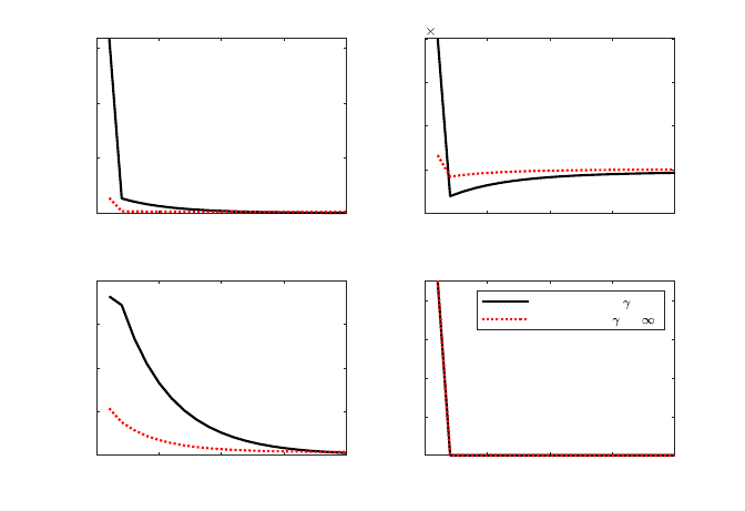
V.1. Reducing local bank RR. Figure 4 displays the impulse responses to a 1% negative
RR shock on local banks (ϵ
l
τ,t
= −0.01). Reducing τ
l
lowers the local banks’ funding cost
and thus their required return on lending. However, reducing τ
l
also leads local banks to
hold less riskless bank reserves and raise local banks’ probability of insolvency. The increase
in the probability of local banks’ insolvency raises the overvaluation distortion on local bank
lending and eases their lending terms. As local banks expand their credit supply, the national
banking sector shrinks and the liquidity services provided by national banks become more
valuable. This reduces the national bank deposit rate and the probability of national bank
insolvency.
In the case with no switching costs (γ = 0), reducing τ
l
lowers the interest charged by
local banks’ on lending, and leads some firms to switch their borrowing from national banks
to local banks. Since local banks have superior monitoring technology and are willing to
accept riskier borrowers, the shift to local banks raises average firm leverage and default
ratios. As a result, firms’ leverage and output are increased. However, firm default costs
and local bank bankruptcy costs also increase.
In the case with infinite switching costs (γ = +∞), reducing τ
l
also lowers the local
banks’ required return on lending, and firms again respond by increasing their leverage
and raising output. However, compared with the case with no switching costs (γ = 0), the
stimulative impact is much weaker because the restrictions against switching banks eliminates
the expansionary extensive-margin effect.
V.2. Reducing national bank RR. Figures 5 displays the impulse responses to a 1%
negative RR shock on national banks (ϵ
n
τ,t
= −0.01). In the case with no switching costs
(γ = 0), cutting τ
n
has two opposite effects: At the intensive margin, it lowers national
banks’ required return on lending falls, which and encourages increased firms borrowing
from national banks to take on more leverage. At the extensive margin, firms shift from local
banks to national banks. This lowers the average firm leverage ratio as local banks’ superior
TARGETED RESERVE REQUIREMENTS 21
0 5 10 15 20
0
0.5
1
1.5
Local bank loan share
0 5 10 15 20
-5
0
5
10
15
10
-3
GDP
0 5 10 15 20
0
0.01
0.02
0.03
0.04
Average firm debt ratio
0 5 10 15 20
0
0.1
0.2
0.3
0.4
Local bank insolvency ratio
Free switching ( = 0)
No switching ( = + )
Figure 4. Impulse responses of a 1% negative RR shock on local banks (ϵ
l
τ,t
=
−0.01). Black solid lines: no switching costs (γ = 0); red dotted lines: infinite
switching costs (γ = +∞). The horizontal axes show the quarters after the
impact period of the shock. The horizontal axes show the quarters after the
impact period of the shock. The units on the vertical axes are percentage-point
deviations from the steady state levels for local bank insolvency ratio. The
units on the vertical axes are percent deviations from the steady state levels
for other variables.
monitoring technologies induce them to accept riskier borrowers. Under our calibration, the
extensive-margin effect dominates and cutting τ
n
leads to a fall in total output.
In the case with infinite switching costs (γ = +∞), firms do not switch between banks,
so the extensive-margin effect no longer operates. Cutting τ
n
raises national bank lending,
reducing firm funding costs and raising output.
VI. Business cycle analysis for China RR policy
In this section, we consider the dynamic implications of pursued RR policy in China in
the wake of adverse technology shocks. We characterize China RR policy in terms of two
alternative feedback rules which the central bank follows in response to deviations of the real
GDP from its trend. One rule is assumed to prevail under normal conditions, and the other
is adopted in response to deep downturns. We compare these dynamics to a benchmark
regime where RR of both types of banks are kept constant at their steady state levels over
the course of the cycle.

TARGETED RESERVE REQUIREMENTS 22
0 5 10 15 20
-1.5
-1
-0.5
0
Local bank loan share
0 5 10 15 20
-10
-5
0
5
10
-3
GDP
0 5 10 15 20
-0.03
-0.02
-0.01
0
0.01
Average firm debt ratio
0 5 10 15 20
-5
0
5
10
15
10
-4
Local bank insolvency ratio
Free switching ( = 0)
No switching ( = + )
Figure 5. Impulse responses of a 1% negative RR shock on national banks
(ϵ
n
τ,t
= −0.01). Black solid lines: no switching costs (γ = 0); red dotted lines:
infinite switching costs (γ = +∞). The horizontal axes show the quarters after
the impact period of the shock. The horizontal axes show the quarters after
the impact period of the shock. The units on the vertical axes are percentage-
point deviations from the steady state levels for local bank insolvency ratio.
The units on the vertical axes are percent deviations from the steady state
levels for other variables.
Under our calibration, firms borrow from both types of banks and are indifferent between
the two types of banks in the initial steady state. As is implied by (A1), they switch across
banks only when the economy is hit by a sufficiently large shock that the improvement in
the their return to equity of switching from one bank to another exceeds the switching cost.
This implies that our model contains occasionally binding constraints.
9
VI.1. RR rules. The central bank adjusts the required reserve ratio (τ
n,t
or τ
l,t
) to respond
to deviations of real GDP from trend.
τ
l,t
= ¯τ
l
+ ψ
ly
ln
˜
GDP
t
(46)
τ
n,t
= ¯τ
n
+ ψ
ny
ln
˜
GDP
t
(47)
9
We solve the model using a popular model solution toolbox called OccBin developed by Guerrieri and
Iacoviello (2015). The toolbox adapts a first-order perturbation approach and applies it in a piecewise fashion
to solve dynamic models with occasionally binding constraints.

TARGETED RESERVE REQUIREMENTS 23
where the parameters ψ
ly
and ψ
ny
measure the responsiveness of the require reserve ratios
to the output gap.
We first consider a symmetric RR rule which characterizes PBOC policy under normal
conditions, under which the reaction coefficients satisy ψ
ly
= ψ
ny
= 1. We estimate the value
of the reaction coefficient by regressing the RRs on the real GDP gap and the CPI inflation
rate using Chinese quarterly data from 2000 to 2020.
Our second RR rule is asymmetric, under which the RR reaction coefficients ψ
ly
= 2 and
ψ
ny
= 0, and reflects pursued PBOC policy in the wake of deep adverse shocks. Under this
rule, the central bank aggressively cuts RRs on local banks in response to downturns but
only modestly adjusts RRs on national banks. This fits the pattern of pursued policy during
the recent coronavirus pandemic.
10
VI.2. Macro implications.
VI.2.1. Large shocks versus small shocks. To begin with, we explore the macro implications
of technology shocks with different shock sizes in a benchmark regime where RR of both
types of banks are kept constant at their steady state levels. Figure 6 compares the impulse
responses of a relatively small negative technology shock ϵ
at
= −0.01 and a relatively large
negative technology shock ϵ
at
= −0.05 in the benchmark regime.
We first focus on a relatively small negative technology shock ϵ
at
= −0.01, whose responses
are shown in black solid lines. The negative technology shock reduces firms’ return to
investment, imposing upward pressure on firm default possibilities and credit spreads at
existing lending levels. In response to higher spreads and reduced profitability, firms respond
by reducing their leverage ratio. This leads to reduced returns on equity.
Firms that borrow from local banks are more negatively affected than those that borrow
from national banks. Local banks, due to their monitoring advantages, have higher steady
state leverage and default probabilities. This leaves local bank terms more sensitive to ad-
verse shocks than national banks. However, under the small technology shock the switching
cost is too high, precluding firms borrowing from local banks from switching to national
banks.
Alternatively, consider a relatively large negative technology shock ϵ
at
= −0.05, whose
responses are shown in red dotted lines. the negative technology shock reduces all firms’
return to equity, although more acutely for firms borrowing from local banks. In this case,
the improvement in returns to equity from switching to national banks are large enough to
10
As shown in Figure 1, the PBOC dropped RR for both large banks as well as medium and small banks
during the 2008 global financial crisis. However, it dropped those for medium and small banks far more
aggressively than it did for large banks, in line with the asymmetry pursued during the pandemic.

TARGETED RESERVE REQUIREMENTS 24
0 10 20
-6
-4
-2
0
GDP
0 5 10 15 20
0
1
2
Change in the share of national bank borrowers’ net worth caused by firm switching
0 10 20
-10
-5
0
Total bank loan
0 10 20
-15
-10
-5
0
Local bank loan
0 10 20
-6
-4
-2
0
National bank loan
Small shock
Large shock
Figure 6. Impulse responses to a small negative technology shock (ϵ
at
= −0.01, black
solid lines) and to a large negative technology shock (ϵ
at
= −0.05, red dotted lines). The
horizontal axes show the quarters after the impact period of the shock. The units on the
vertical axes are percentage-point deviations from the steady state levels for the variable
“Change in the share of national bank borrowers’ net worth caused by firm switching,”
which, denoted by
N
n,t
−
¯
N
n,t−1
¯
N
t−1
, refers to the ratio of the net worth of firms that switch from
local banks to national banks to the net worth of all firms. The units on the vertical axes
are percent deviations from the steady state levels for other variables.
cover the switching cost for some local bank borrowers. As a result, while total lending falls,
national bank lending rises relative to local bank lending. The shift to national banks also
lowers the average leverage ratio, further reducing total lending and output.
An important take-away from Figure 6 is that local banks’ credit supply are more cycli-
cally sensitive than national banks. Furthermore, this extra sensitivity is larger in times of
large shocks, attributed to firm switching across the two types of banks. These results are
supported by the empirical evidence using Chinese bank-level data, which we will show later
in Section VII.
VI.2.2. Symmetric versus asymmetric RR rule under small shocks. Figure 7 displays the
impulse responses to a relatively small negative technology shock ϵ
at
= −0.01 under alter-
native policy rules. With no switching taking place, the decline in aggregate TFP leads to
a fall in real GDP. In this case, the symmetric RR policy and the asymmetric RR policy are
almost equally effective in stabilizing the output. In particular, the RR cut on both types
of banks under the symmetric rule reduces the funding costs of both types of banks and
mitigates the fall in real GDP by raising credit supply in both banking sectors. In contrast,
the asymmetric cut that only reduces RR on local banks stimulates the credit supply by
local banks but tightens the credit supply by national banks.

TARGETED RESERVE REQUIREMENTS 25
0 10 20
-1
-0.9
-0.8
-0.7
GDP
0 5 10 15 20
-0.01
0
0.01
Change in the share of national bank borrowers’ net worth caused by firm switching
0 10 20
-2
-1.5
-1
-0.5
Total bank loan
0 10 20
-4
-2
0
2
Local bank loan
0 10 20
-2
-1.5
-1
-0.5
National bank loan
Benchmark
Symmetric RR policy
Asymmetric RR policy
Figure 7. Impulse responses to a small negative technology shock (ϵ
at
= −0.01) under
alternative policy rules. Benchmark rule: black solid lines; symmetric RR rule: blue dashed
lines; assymmetric rule: red dotted lines. The horizontal axes show the quarters after the
impact period of the shock. The units on the vertical axes are percentage-point deviations
from the steady state levels for the variable “Change in the share of national bank borrowers’
net worth caused by firm switching.” The units on the vertical axes are percent deviations
from the steady state levels for other variables.
VI.2.3. Symmetric versus asymmetric RR rule under large shocks. Figure 8 displays the
impulse responses to a large negative technology shock ϵ
at
= −0.05 under alternative policy
rules. Given the large shock, the RR cut on both types of banks helps to reduce all banks’
funding costs and mitigates the fall in the real GDP. However, the asymmetric cut stabilizes
real GDP better than cutting RRs symmetrically across bank types. This is because the
asymmetric RR cut lowers the local bank lending rate relative to that of national banks,
preventing firms switching to national banks and taking lower leverages. By comparison,
while the symmetric cut stimulates both types of bank lending, it does not raise the total
credit as much because firms switch to national banks.
VI.3. Macro stability versus financial stability. In our model, as is shown in (41),
the GDP is defined as the gross output net of the resource costs for monitoring defaulting
firms, liquidating insolvent local banks, and switching borrowers. Therefore, to stabilize the
GDP, the government needs to lessen the fluctuations not only in the gross output, which
could be achieved by stabilizing firms’ borrowing and production activities, but also of the
resource costs associated with various financial activities. We now compare the symmetric
and asymmetric RR policies in terms of their performance in stabilizing the gross output as
well as the financial resource costs.

TARGETED RESERVE REQUIREMENTS 26
0 10 20
-5
-4.5
-4
-3.5
GDP
0 5 10 15 20
-5
0
5
Change in the share of national bank borrowers’ net worth caused by firm switching
0 10 20
-10
-5
0
Total bank loan
0 10 20
-20
0
20
40
Local bank loan
0 10 20
-30
-20
-10
0
National bank loan
Benchmark
Symmetric RR policy
Asymmetric RR policy
Figure 8. Impulse responses to a large negative technology shock (ϵ
at
= −0.05) under
alternative policy rules. Benchmark rule: black solid lines; symmetric RR rule: blue dashed
lines; assymmetric rule: red dotted lines. The horizontal axes show the quarters after the
impact period of the shock. The units on the vertical axes are percentage-point deviations
from the steady state levels for the variable “Change in the share of national bank borrowers’
net worth caused by firm switching.” The units on the vertical axes are percent deviations
from the steady state levels for other variables.
Table 2 displays the total fluctuations in the GDP and its determinants in response to
negative technology shocks with different shock sizes, calculated as the sum of the deviation
of the corresponding variable to its steady-state level on each quarter after the impact period
of the shock and expressed as a fraction of the steady-state GDP level.
Under the benchmark regime with constant RRs, a 1% negative technology shock reduces
the gross output by 46.44% and the GDP by 45.87%. The smaller fall in the GDP is
attributed to the decline in financial activities, reducing the cost from monitoring default
loans by 0.5% and the cost from liquidating insolvent local banks by 0.07%. For a larger
shock (5% negative technology shock), the fluctuations in the GDP and its determinants are
similar, except that firms begin to switch between banks. In this case, the extensive-margin
effect from bank switching exaggerates the output fluctuations and incurs a very small firm
switching cost that equals 0.004% of steady state GDP.
We now consider the performance of the symmetric and asymmetric RR policies relative
to the benchmark regime. Table 2 shows that, the asymmetric RR adjustments on local
banks are more efficient in stabilizing the gross output than the symmetric RR adjustments.
This difference is also larger under larger shocks. The reason is demonstrated in our impulse
responses, as the more aggressive cut of RR on local banks relative to national banks helps
reverse the firm switching from local banks to national banks and thus better stabilizes total
lending through the extensive-margin effect during severe economic downturns.

TARGETED RESERVE REQUIREMENTS 27
Table 2. Total fluctuations in the GDP and its determinants in response to negative
technology shocks
Total fluctuations Relative to the benchmark regime
Benchmark Symmetric RR Asymmetric RR Symmetric RR Asymmetric RR
Responses to a 1% negative technology shock
GDP −45.87 −44.66 −42.55 1.20 3.32
Gross output −46.44 −44.88 −42.11 1.57 4.33
Cost from firm switching 0 0 0 0 0
Cost from default loans −0.50 −0.35 −0.22 0.15 0.28
Cost from insolvent banks −0.07 0.14 0.66 0.21 0.74
Local bank insolvency ratio 0.09 20.32 38.64 20.24 38.56
Responses to a 5% negative technology shock
GDP −231.60 −224.22 −206.51 7.38 25.10
Gross output −234.92 −225.48 −202.69 9.45 32.24
Cost from firm switching 0.004 0.002 0.058 −0.002 0.054
Cost from default loans −2.59 −1.80 −0.86 0.79 1.73
Cost from insolvent banks −0.73 0.55 4.62 1.28 5.35
Local bank insolvency ratio 0.43 102.02 187.55 101.59 187.12
Note: This table displays total fluctuations in the GDP and its determinants in response to
negative technology shocks with different shock sizes, calculated as the sum of the deviation of
the corresponding variable to its steady-state level on each quarter after the impact period of
the shock and expressed as a fraction of the steady-state GDP level in percentage points. These
variables include GDP GDP
t
, gross output Y
t
, cost from firm switching
P
b=n,l
γ max{N
b,t
−
¯
N
b,t−1
, 0}, cost from default loans
P
b=n,l
˜
A
t
(N
b,t
+ B
b,t
)m
b
R
ω
bt
0
ωdF (ω), cost from insolvent
banks µ
l
R
¯ϵ
l,t
0
ϵ
l,t
R
l,t
b
l,t
dΦ(ϵ
l,t
). The table also displays total fluctuations in local bank insolvency
ratio F (¯ϵ
l,t
), calculated as the sum of the deviation of the corresponding variable to its steady-
state level on each quarter after the impact period of the shock and expressed in percentage points.
As for financial implications, both the asymmetric RR policy and the symmetric RR
policy incur larger financial resource costs relative to the benchmark regime since these
RR adjustments help mitigate the shrinkage of financial activities under adverse technology
shocks. Under our calibration, the additional cost of liquidating insolvent banks in the
asymmetric RR regime relative to the benchmark regime is relatively large in magnitude
(0.74% and 5.35% for a 1% and 5% negative technology shock), reaching over 16% of the
rise in gross output caused by the asymmetric RR adjustments (4.33% and 32.24% for a
1% and 5% negative technology shock). This is because, in response to adverse technology
shocks, the asymmetric RR cut on local banks leads them to hold less riskless reserves,
raising their insolvency ratio and incurring additional cost of liquidating insolvent local
banks. By comparison, as insolvent national banks could be fully recapitalized without
costly liquidation, the symmetric RR cuts on both types of banks incur less bank insolvency
costs than the asymmetric RR cut on local banks.

TARGETED RESERVE REQUIREMENTS 28
These results illustrate a tradeoff between macro stability and bank insolvency costs when
the government adopts asymmetric RR policies: given adverse technology shocks, the asym-
metric RR cut on local banks helps stabilizes the gross output but incurs larger bank insol-
vency costs by raising the fraction of insolvent local banks, compared with the symmetric RR
cut on both types of banks. Under our calibration, the output stabilizing effect dominates
so that the asymmetric RR policy stabilize the GDP better than the symmetric RR policy,
especially under large shocks. As is shown in Appendix B, this policy tradeoff is arises under
alternative calibrated values of the firm switching cost parameter γ, the bank liquidation
cost parameter µ
l
, as well as under alternative values of RR policy reaction coefficients and
technology shock sizes.
VII. Empirical evidence
In our model, small banks, due to their monitoring advantages, allow for higher firm
leverage and default probabilities in the steady state than large banks. As a consequence,
small bank lending is more responsive to business cycle fluctuations than large bank lending.
Furthermore, sufficiently large shocks may disrupt banking relationships and increase the
discrepancy between small and large bank lending volatility, implying that asymmetric RR
on the two types of banks can facilitate macroeconomic stabilization. In this section, we
show that these disparities in large and small bank lending sensitivities to business cycle
movements are consistent with empirical evidence for banks in China.
VII.1. Methodology. China’s commercial banking sector consists of six large-sized state-
owned banks
11
, twelve joint-stock banks, and a large number of medium-sized urban banks
and small-sized rural banks. Differences in bank size are primarily attributable to the dif-
ferences in operating areas: While the six large-sized state-owned banks have branches na-
tionwide, small commercial banks usually concentrate their lending in a specific area. In
particular, rural banks are restricted to focus their lending activity within certain county-
level towns or villages. In contrast, urban banks are less focused than rural banks as they are
allowed to operate within a province or a prefectural-level city, which usually includes a main
central urban area and its surrounding rural areas. Finally, joint-stock banks have national
operating licenses and are allowed to operate nationally. However, most joint-stock banks
are evolved from urban banks and usually concentrate their lending in one area comparable
in size to those of urban banks.
As discussed above, China banks also are subject to different policy treatment by group,
including PBoC discrimination across banks by size in RR. To identify the implications of
11
These six banks are Agricultural Bank of China, Bank of China, Bank of Communications, China
Construction Bank, Industrial and Commercial Bank of China and Postal Savings Bank of China.

TARGETED RESERVE REQUIREMENTS 29
these policy treatment differences, we consider a sample of banks subject to different local
economic shocks. Specifically, we focus on medium-sized and small-sized commercial banks,
dropping the six large-sized commercial banks from our sample because their loan portfolios
are diversified nationally. We compare how these two groups of banks respond differently to
regional economic shocks using the following empirical specification:
∆L
i,t
= c + β∆Y
j(i),t
× SM
i
+ β
x
X
i,t−1
+ θ
t
+ Z
i
+ P
j
× θ
t
+ SM
i
× θ
t
+ ϵ
i,t
(48)
where the dependent variable ∆L
i,t
denotes the growth rate in bank i’s loan from year
t − 1 to year t. ∆Y
j(i),t
denotes the real GDP growth in province j(i) in year t, where j(i)
denotes the province where bank i’s headquarter locates. SM
i
is a dummy variable that
equals one if bank i is a rural bank, and zero if bank i is an urban bank or a joint-stock
bank. X
i,t−1
denotes a battery of control variables to control for bank-specific characteristics
that may influence bank lending over our sample. This set of control variables use lagged
values and includes the deposit to asset ratio D/A
i,t−1
, the equity to asset ratio E/A
i,t−1
, the
non-performing loan ratio NP L
i,t−1
, the interest income and fees to asset ratio INT/A
i,t−1
,
and the loan to asset ratio L/A
i,t−1
.
12
θ
t
, Z
i
and P
j
represents year, bank and province
dummies, respectively. We include province-year dummies P
j
× θ
t
to control for potential
endogenous co-movements between bank loan and real GDP at the province level. We also
include interaction between small-bank dummies SM
i
and the year dummies θ
t
to control
for the impacts from differential policy treatments based on bank size at the national level.
Note that we do not include province dummies P
j
or small-bank dummies SM
i
in the above
specification because they are collinear with the bank dummies Z
i
in our sample.
In our baseline specification (48), we use province-specific real GDP growth ∆Y
j(i),t
to
capture the variations in local economic conditions that affect the market equilibrium of
bank loans. The dummy variable SM
j
is used to distinguish small-sized banks (SM
i
= 1)
from medium-sized banks (SM
i
= 0). The coefficient of interest is β, the coefficient on the
interaction between these two variables. In particular, β captures the additional sensitivity
of small banks’ loan growth to changes in local real GDP growth and should be positive
based on our model.
VII.2. Data. We obtain Chinese bank-level data and province-level data from China Stock
Market & Accounting Research Database (CSMAR). Our bank-level dataset is an unbalanced
panel of 320 small-sized commercial banks and 142 medium-sized commercial banks at the
annual frequency over a sample period from 2008 to 2021. The number of banks in our
sample starts from 92 in 2008, reaches 448 in 2019 and ends with 350 in 2021, with bank
12
Here, ”assets” refers to book value of total assets.

TARGETED RESERVE REQUIREMENTS 30
Table 3. Summary Statistics
Full sample Small-sized banks (SM
i
= 1) medium-sized banks (SM
i
= 0)
N Mean Std. Dev. N Mean Std. Dev. N Mean Std. Dev.
∆L
i,t
3,685 0.18 0.12 2,155 0.15 0.11 1,530 0.22 0.13
D/A
i,t
2,893 0.78 0.98 1,442 0.86 1.38 1,451 0.71 0.12
E/A
i,t
2,903 0.08 0.03 1,451 0.09 0.03 1,452 0.07 0.02
NP L
i,t
3,668 1.89 1.32 2,145 2.20 1.47 1,523 1.45 0.90
INT/A
i,t
2,877 0.05 0.01 1,430 0.05 0.01 1,447 0.05 0.02
L/A
i,t
2,894 0.52 0.58 1,443 0.59 0.81 1,451 0.45 0.11
∆Y
j(i),t
4,458 0.08 0.03 2,771 0.08 0.02 1,687 0.08 0.03
Note: This table displays summary statistics of our bank-level sample used in the baseline
regression. It also displays summary statistics for small-sized commercial banks (SM
i
=
1) and for medium-sized commercial banks (SM
i
= 0). The bank-level variables include
bank loan growth ∆L
i,t
, deposit to asset ratio D/A
i,t
, equity to asset ratio E/A
i,t
,
nonperforming loan ratio N P L
i,t
, interest income and fees to asset ratio INT/A
i,t
, loan
to asset ratio L/A
i,t
. N is the number of non-missing observations in the sample for each
variable.
Source: China Stock Market & Accounting Research Database (CSMAR).
entry and exit in each year. Table 3 displays the summary statistics of our bank-level sample,
which we have winsorized at the 1% level to ensure that our results are not driven by outliers.
We also display the summary statistics for small-sized commercial banks and medium-sized
commercial banks separately. Table 3 shows that means of banking characteristics measures
for the two types of banks in our sample are comparable, although standard deviations of
characteristics are generally larger for the small bank group.
Our province-level data provides the province-specific real GDP growth ∆Y
j,t
used in our
regression and is a balanced panel of 29 province-level regions that cover the headquarter
location of all the banks in our bank-level sample. The province-level data is also winsorized
at the 1% level.
Table 4 shows how our bank-level sample is distributed across location regions and bank
size types. We can see that our bank-level sample displays significant heterogeneity in
location regions. In particular, even the region that is located by most banks (69 banks) and
has the largest number of bank-year observations (715), the Fujian province, only accounts
for around 15% of 462 banks and 715 bank-year observations in the full bank-level sample.
VII.3. Baseline estimates. We report the estimation results under our baseline specifica-
tion (48) using the full sample in Table 5 Column 1. The estimated value of β is positive
and statistically significant at the 5% level, consistent with our model’s prediction. The
estimated value of β is also economically significant. Our point estimate indicates that a one
percentage point increase in the real GDP growth would increase the loan growth rate of an
average small-sized commercial bank relative to a medium-sized commercial bank by 1.212
percentage point.

TARGETED RESERVE REQUIREMENTS 31
Table 4. Sample distribution by location region and bank
size type
Number of banks Number of bank-year observations
Region name SM
i
= 1 SM
i
= 0 Total SM
i
= 1 SM
i
= 0 Total
Fujian 64 5 69 649 63 712
Zhejiang 33 13 46 352 173 525
Jiangsu 38 4 42 397 51 448
Anhui 45 1 46 425 14 439
Guangdong 24 8 32 205 100 305
Sichuan 19 14 33 120 157 277
Shandong 5 15 20 35 201 236
Jiangxi 20 3 23 147 42 189
Liaoning 6 12 18 41 136 177
Henan 12 12 24 58 83 141
Hebei 8 10 18 24 108 132
Beijing 2 5 7 22 70 92
Hunan 11 2 13 54 26 80
Shanxi 4 6 10 16 60 76
Inner Mongolia 7 3 10 31 35 66
Hubei 4 2 6 37 25 62
Guangxi 2 3 5 18 42 60
Chongqing 3 2 5 29 27 56
Shaanxi 3 2 5 21 26 47
Shanghai 1 2 3 14 28 42
Tianjin 1 2 3 12 28 40
Ningxia 1 2 3 13 26 39
Guizhou 2 2 4 17 21 38
Yunnan 0 3 3 0 38 38
Jilin 2 1 3 21 13 34
Xinjiang 2 3 5 2 32 34
Heilongjiang 0 2 2 0 26 26
Qinghai 1 1 2 11 13 24
Gansu 0 2 2 0 23 23
Total 320 142 462 2,771 1,687 4,458
Note: Each row of this table shows the number of banks and the num-
ber of bank-year observations for a subsample of banks whose head-
quarter locates in a given province-level region. The table also displays
the number of banks and the number of bank-year observations for
small-sized commercial banks (SM
i
= 1) and for medium-sized com-
mercial banks (SM
i
= 0).

TARGETED RESERVE REQUIREMENTS 32
Table 5. Regression results.
Sample (1) Full
D = 0.04 D = 0.03 D = 0.05
(2) Small shock (3) Large shock (4) Small shock (5) Large shock (6) Small shock (7) Large shock
∆Y
j(i),t
× SM
i
1.212
∗∗
1.318 2.995
∗∗
1.196 3.404
∗∗∗
1.333
∗
10.183
∗∗∗
(0.584) (0.830) (1.416) (0.989) (1.223) (0.798) (2.113)
D/A
i,t−1
0.395
∗∗∗
0.398
∗∗∗
0.162 0.396
∗∗∗
0.173
∗
0.396
∗∗∗
0.304
∗∗∗
(0.049) (0.060) (0.112) (0.064) (0.105) (0.057) (0.106)
E/A
i,t−1
1.070
∗∗∗
1.104
∗∗∗
1.551
∗∗∗
1.092
∗∗∗
1.321
∗∗∗
1.087
∗∗∗
2.619
∗∗∗
(0.189) (0.209) (0.546) (0.216) (0.411) (0.201) (0.661)
NP L
i,t−1
−0.007
∗∗
−0.007
∗∗
−0.022 −0.007
∗∗
−0.004 −0.007
∗∗
−0.016
(0.003) (0.003) (0.024) (0.004) (0.007) (0.003) (0.029)
INT/A
i,t−1
−0.503
∗∗∗
−0.764 −0.668
∗∗∗
−1.011
∗
−0.528
∗∗∗
−0.579
∗∗∗
8.865
∗∗∗
(0.188) (0.518) (0.101) (0.540) (0.179) (0.185) (1.901)
L/A
i,t−1
−0.665
∗∗∗
−0.668
∗∗∗
−0.559
∗∗∗
−0.663
∗∗∗
−0.663
∗∗∗
−0.666
∗∗∗
−0.415
∗∗
(0.085) (0.103) (0.112) (0.110) (0.112) (0.098) (0.189)
Constant 0.193
∗∗∗
0.195
∗∗∗
0.579
∗
0.211
∗∗∗
0.247
∗∗
0.190
∗∗∗
−0.373
(0.042) (0.049) (0.303) (0.049) (0.119) (0.045) (0.238)
Sample size 2706 2291 415 2103 603 2412 294
Adjusted R-square 0.37 0.36 0.72 0.33 0.58 0.37 0.78
Note: The dependent variable is ∆L
i,t
in all specifications. Bank dummies Z
i
, year dummies θ
t
, province-year dummies
P
j
× θ
t
, small-bank-year dummies SM
i
× θ
t
are included in all specifications. Column (1) reports the estimates using the
full sample. Columns (2)-(7) separate the sample into sub-samples of small and large shocks. A bank-year observation
is classified in the large (small) shock subsample if the bank locates in the province whose real GDP growth in current
year deviates from its historical average by more (less) than a threshold level D, where the benchmark D = 0.04 value
is chosen to minimize oot-of-sample MSE and the alternative values are included for robustness checks. Standard
errors clustered at the bank level are shown in parentheses. Statistical significance levels are indicated by the asterisks:
∗∗∗
: p < 0.01,
∗∗
: p < 0.05, and
∗
: p < 0.10.

TARGETED RESERVE REQUIREMENTS 33
Figure 9. Fraction of banks that are classified as experiencing a ”large shock” in each
year over the sample period 2008 to 2021. A bank-year observation is classified in the
large (small) shock subsample if the bank locates in the province whose real GDP growth
in current year deviates from its historical average by more (less) than a threshold level
D = 0.04.
VII.4. Subsample estimates. Our model also predicts that the disparity between large
and small bank sensitivity is larger in times of sufficiently large shocks. To show this, we
estimate our baseline specification (48) in two sub-samples: a ”large shock” sub-sample and
a ”small shock” sub-sample. The classification is based on how much the province-specific
real GDP growth ∆Y
j,t
deviates from its historical average ∆Y
j
≡
1
15
P
2021
t=2007
∆Y
j,t
. In
particular, we classify a bank i in a given province j(i) as experiencing large shocks in year t
if the province-specific real GDP growth deviates from its historical average by more than a
threshold level D (i.e. |∆Y
j,t
− ∆Y
j
| > D), and in the ”small shock” sub-sample if otherwise
(i.e. |∆Y
j,t
− ∆Y
j
| ≤ D). We set the threshold level D to minimize out-of-sample mean
squared error based on the sub-sample estimates.
13
In this way, we obtains D = 0.04 as a
benchmark, which is around 1.3 times the standard deviation of China’s national real GDP
growth over our sample period. To check the robustness of our results, we also consider two
alternative thresholds for large shocks, D = 0.03 and D = 0.05.
Figure 9 shows the fraction of banks that are classified as experiencing a ”large shock” in
our sample. Most of the ”large shock” observations occur during the 2007 global financial
crisis and the recent Covid pandemic in 2020, precisely the periods in which the PBoC
implements targeted RR adjustments based on bank size.
13
Appendix C provides details on the calculation of the out-of-sample mean squared error and reports its
values for various threshold levels of D.
TARGETED RESERVE REQUIREMENTS 34
We report the estimation results under our baseline specification (48) for the two subsam-
ples in Table 5 Column 2 and 3. The estimated value of β is not significant from zero in the
”small shock” sample but becomes significantly positive in the ”large shock” sample. The
value of β estimated in the ”large shock” sample is around 2.5 times as large as the full-sample
estimate shown in Column 1. These results suggest that, compared with medium-sized com-
merical banks, small-sized commerical banks’ lending activities are particularly sensitive to
local economic growth in times of large shocks.
The empirical evidence is robust to alternative definitions of large shocks. Table 5 Column
4-7 reports the estimation results when we change the threshold level to D = 0.03 or D =
0.05. The value of β estimated in the ”large shock” sample is still significantly larger than
the ”small shock” estimate. Notably, when we tighten the criterion to identify large shocks
by raising the threshold level to D = 0.05, the value of β estimated for the ”large shock”
sample (shown in Column 7) become almost 10 times as large as the full-sample estimate
(shown in Column 1).
VII.5. Robustness. Our results are robust to a number of sensitivity checks, which are
reported in Appendix D. First, We examine the robustness of our results to the use of
unwinsorized data, which is shown in Table D1 and obtain qualitatively similar results as
those in our baseline regressions. Notably, the estimate value of β for the ”large shock”
sample is extremely large (104.5) when a relatively high threshold level (D = 0.05) is used.
This result further verifies our model’s mechanism where, in times of sufficiently large shocks,
costly disruption of banking relationships could dramatically raise the extra business cycle
sensitivity of small banks, thus generating outliers in the data. Second, We re-estimate our
baseline specification with standard errors clustered at the province level instead of the firm
level. Table D2 shows that such variation also does not change our qualitative results.
TARGETED RESERVE REQUIREMENTS 35
VIII. Conclusion
We have studied the effectiveness of targeted changes in reserve requirement policy as
a macroeconomic stabilization tool, a policy that has been implemented by China during
the global financial crisis and the COVID-19 pandemic. We present a theoretical model in
which firms can borrow from either local banks, which have access to superior monitoring
technologies, or national banks that provide superior liquidity services and thus face lower
funding costs. Borrowers can switch bank types by paying a fixed cost. Thus, costly bank
switching only occurs under sufficiently large shocks.
Our model implies that targeted RR policy helps stabilize macroeconomic fluctuations,
especially when the economy is buffeted by large shocks. Under such policy, the central
bank cuts RR more aggressively for local banks than for national banks in response to a
large decline in output gap. This policy mitigates costly bank switching in deep recessions
and helps to stabilize macroeconomic fluctuations. However, this macroeconomic stability
gain comes with a financial stability cost, since the policy boosts local bank leverage, raising
default risks and liquidation losses.
The model mechanism and the its predictions are in line with empirical evidence. Con-
sistent with our theory, bank-level evidence suggests that lending growth by small banks
is on average more sensitive to local shocks than lending growth by medium-sized banks.
Furthermore, when the shocks are large, small lending responds significantly more than
medium-sized bank lending.
References
Ag´enor, P´ıerre-Richard, Koray Alper, and Luiz Pereira da Silva, “External shocks,
financial volatility and reserve requirementsin an open economy,” Journal of International
Money and Finance, 2018, 83, 23–43.
Alper, Koray, Mahir Binici, Selva Demiralp, Hakan Kara, and Pinar
¨
Ozl¨u, “Re-
serve Requirements, Liquidity Risk, and Bank Lending Behavior,” Journal of Money,
Credit and Banking, 2018, 50 (4), 817–827.
Angelini, Paolo, Stefano Neri, and Fabio Panetta, “The Interaction between Capital
Requirements and Monetary Policy,” Journal of Money, Credit and Banking, September
2014, 46 (6), 1073–1112.
Begenau, Juliane, “Capital requirements, risk choice, and liquidity provision in a business-
cycle model,” Journal of Financial Economics, 2020, 136, 355–378.
Bernanke, Ben, Mark Gertler, and Simon Gilchrist, “The Financial Accelerator in a
Quantitative Business Cycle Framework,” in John B. Taylor and Michael Woodford, eds.,
TARGETED RESERVE REQUIREMENTS 36
Handbook of Macroeconomics, Amsterdam, New York, and Oxford: Elsevier Science, 1999,
pp. 1341–1393.
Boot, Arnoud W. A., “Relationship Banking: What Do We Know?,” Journal of Financial
Intermediation, January 2000, 9 (1), 7–25.
Brandt, Loren, Chang-Tai Hsieh, and Xiaodong Zhu, “Growth and Structural Trans-
formation in China,” in Loren Brandt and Thomas G. Rawski, eds., China’s Great Eco-
nomic Transformation, Cambridge University Press, 2008, pp. 683–728.
Brei, Michael and Ramon Moreno, “Reserve requirements and capital flows in Latin
America,” Journal of International Money and Finance, 2019, 99, 1–20.
Chang, Chun, Zheng Liu, Mark M. Spiegel, and Jingyi Zhang, “Reserve require-
ments and optimal Chinese stabilization policy,” Journal of Monetary Economics, 2019,
103, 35–51.
Christiano, Lawrence and Daisuke Ikeda, “Bank leverage and social welfare,” American
Economic Review, 2016, 106 (5), 560–564.
Christiano, Lawrence J., Martin Eichenbaum, and Charles L. Evans, “Nominal
Rigidities and the Dynamic Effects of a Shock to Monetary Policy,” Journal of Political
Economy, 2005, 113 (1), 1–45.
Corbae, Dean and Pablo D’Erasmo, “Capital Requirements in a quantiative model of
banking industry dynamics,” January 2019. NBER Working Paper 25424.
den Heuvel, Skander J. Van, “The welfare cost of bank capital requirements,” Journal
of Monetary Economics, 2008, 55, 196–233.
d’Avernas, Adrien, Andrea L. Eisfeldt, Can Huang, Richard Stanton, and Nancy
Wallace, “The Deposit Business at Large vs. Small Banks,” October 2023. Unpublished
manuscript.
Federico, Pablo, Carlos A. Vegh, and Guillermo Vuletin, “Reserve Requirement
Policy Over the Business Cycle,” October 2014. NBER Working Paper No. 20612.
Gerali, Andrea, Stefano Neri, Luca Sessa, and Federico M. Signoretti, “Credit and
Banking in a DSGE Model of the Euro Area,” Journal of Money, Credit and Banking,
September 2010, 42 (s1), 107–141.
Gertler, Mark and Nobuhiro Kiyotaki, “Financial Intermediation and Credit Policy in
Business Cycle Analysis,” in Benjamin M. Friedman and Michael Woodford, eds., Hand-
book of Monetary Economics, Vol. 3 of Handbook of Monetary Economics, Elsevier, 2010,
chapter 11, pp. 547–599.
Glocker, Christian and Pascal Towbin, “Reserve requirements as a macroprudential
instrument - Empirical evidence from Brazil,” Journal of Macroeconomics, 2015, 44, 158–
176.
TARGETED RESERVE REQUIREMENTS 37
G´ornicka, Lucyna A., “Banks and shadow banks: Competitors or complements?,” Journal
of Financial Intermediation, 2016, 27, 118–131.
Gorton, Gary, Stefan Lewellen, and Andrew Metrick, “The safe asset share,” Amer-
ican Economic Review, 2012, 102 (3), 101–106.
Guerrieri, Luca and Matteo Iacoviello, “OccBin: A toolkit for solving dynamic models
with occasionally binding constraints easily,” Journal of Monetary Economics, 2015, 70
(C), 22–38.
Hsieh, Chang-Tai and Peter J. Klenow, “Misallocation and Manufacturing TFP in
China and India,” The Quarterly Journal of Economics, November 2009, 124 (4), 1403–
1448.
Kashyap, Anil K. and Jeremy C. Stein, “What Do a Million Observations on Banks
Say About the Transmission of Monetary Policy?,” American Economic Review: Papers
and Proceedings, 2000, 90 (3), 2085–2117.
Loungani, Prakash and Mark Rush, “The Effect of Changes in Reserve Requirements
on Investment and GNP,” Journal of Money, Credit and Banking, 1995, 27 (2), 511–526.
Montoro, Carlos and Ramon Moreno, “The Use of Reserve Requirements as a Policy
Instrument in Latin America,” BIS Quarterly Review, March 2011, pp. 53–65.
Mora, Nada, “Microprudential Regulation in a Dynamic Model of Banking,” Journal of
Money, Credit and Banking, March-April 2014, 46 (2-3), 469–501.
Nicol`o, Gianni De, Andrea Gamba, and Marcella Lucchetta, “Microprudential Reg-
ulation in a Dynamic Model of Banking,” Review of Financial Studies, 2014, 27 (7),
2097–2138.
Smets, Frank and Rafael Wouters, “Shocks and Frictions in US Business Cycles: A
Bayesian DSGE Approach,” American Economic Review, 2007, 97 (3), 586–606.
Tovar, Camilo E., Mercedes Garcia-Escribano, and Mercedes Vera Martin,
“Credit Growth and the Effectiveness of Reserve Requirements and Other Macroprudential
Instruments in Latin America,” June 2012. IMF Working Paper WP/12/142.
Ulate, Mauricio, “Going Negative at the Zero Lower Bound: The Effects of Negative
Nominal Interest Rates,” American Economic Review, 2021, 111 (1), 1–40.
Yin, Wei and Kent Matthews, “Why Do Firms Switch Banks? Evidence from China,”
Emerging Markets Finance and Trade, July 2018, 54 (9), 2040–2052.
Zhu, Xiaodong, “Understanding China’s Growth: Past, Present, and Future,” Journal of
Economic Perspectives, 2012, 26 (4), 103–124.
TARGETED RESERVE REQUIREMENTS 38
Appendix A. Changes in aggregate net worth subsequent to switching
banks
Given firms’ optimal choices of the bank type in Eq. (29), the beginning-of-period net
worth is given by
N
l,t
∈ (
¯
N
l,t−1
,
¯
N
t−1
), N
n,t
∈ (0,
¯
N
n,t−1
), if
¯
V
l,t
ROE
l,t
−
¯
V
n,t
ROE
n,t
= γ
¯
V
l,t
,
N
l,t
=
¯
N
l,t−1
, N
n,t
=
¯
N
n,t−1
, if −γ
¯
V
n,t
<
¯
V
l,t
ROE
l,t
−
¯
V
n,t
ROE
n,t
< γ
¯
V
l,t
,
N
l,t
∈ (0,
¯
N
l,t−1
), N
n,t
∈ (
¯
N
n,t−1
,
¯
N
t−1
), if
¯
V
l,t
ROE
l,t
−
¯
V
n,t
ROE
n,t
= −γ
¯
V
n,t
.
(A1)
Eq. (A1) identifies three possible ranges for changes in aggregate net worth subsequent
to switching banks. In the first range, the benefit of switching to a local bank sufficiently
exceeds the benefit of borrowing from a national bank so that some of previous national-bank
borrowers switch to local banks until the benefit of switching from a national bank to a local
banks is driven down to be equal to the cost of switching, i.e.
¯
V
l,t
ROE
l,t
−
¯
V
n,t
ROE
n,t
= γ
¯
V
l,t
.
Such switching behavior raises the aggregate net worth of local-bank borrowers from
¯
N
l,t−1
by the end of previous period t − 1 to N
l,t
at the beginning of period t, and reduces the
aggregate net worth of national-bank borrowers from
¯
N
n,t−1
by the end of previous period
t − 1 to N
n,t
at the beginning of period t. In this case, N
l,t
−
¯
N
l,t−1
≡
¯
N
n,t−1
− N
n,t
> 0
measures the aggregate net worth of firms that switch from a national bank to a local bank.
In the second range, borrowers do not switch banks because the benefit of doing so is less
than the switching cost. As a consequence, the aggregate net worth of each type of borrowers
do not change, i.e. N
l,t
=
¯
N
l,t−1
, N
n,t
=
¯
N
n,t−1
.
The third range is mirror-image of the first, as the benefit of switching to a national bank
sufficiently exceeds the benefit of borrowing from a local bank so that previous local-bank
borrowers switch to national banks until the benefit of switching is again driven down to its
cost, i.e.
¯
V
n,t
ROE
n,t
−
¯
V
l,t
ROE
l,t
= γ
¯
V
n,t
. In this case, the aggregate net worth of firms that
switch from a local bank to a national bank is measured by N
n,t
−
¯
N
n,t−1
≡
¯
N
l,t−1
− N
l,t
> 0.
Eq. (A1) gives the optimal choice of bank type in the interior solution where firms borrow
from both types of banks, which will be the case under our calibration. It is also notable
that, with extreme calibrated values, the gap in the overall return to equity between the two
types of banks could be large enough so that all firms choose the same bank type in a corner
solution:
(
N
l,t
=
¯
N
t−1
, N
n,t
= 0, if
¯
V
l,t
ROE
l,t
−
¯
V
n,t
ROE
n,t
> γ
¯
V
l,t
,
N
l,t
= 0, N
n,t
=
¯
N
t−1
, if
¯
V
l,t
ROE
l,t
−
¯
V
n,t
ROE
n,t
< −γ
¯
V
n,t
.
(A2)
TARGETED RESERVE REQUIREMENTS 39
Appendix B. Robustness checks for business cycle analysis
Section VI.3 illustrates a tradeoff between macro stability and bank insolvency costs when
the government adopts asymmetric RR policies in the presence of adverse technology shocks.
In this Appendix, we demonstrate the robustness of this policy tradeoff to alternative cal-
ibrated values of the firm switching cost parameter γ, the bank liquidation cost parameter
µ
l
, and for alternative values of RR policy reaction coefficients and technology shock sizes,
B.1. Robustness testing on the firm switching cost γ. Figure B1 considers various
sizes of the firm switching cost γ and compares the performance of the symmetric and
asymmetric RR policies relative to the benchmark regime in response to a 1% negative
technology shock.
In the benchmark regime with constant RRs, firms do not switch across banks if the
switching cost is sufficiently high (γ ≥ 0.003). In this case, variations in the size of the firm
switching do not affect the dynamics of the economy. When the firm switching cost γ rises
sufficiently, firms begin to switch between banks, generating an extensive-margin effect that
exaggerate the fluctuations in total credit and output.
Figure B1 shows that the policy tradeoff between macro stability and bank insolvency
costs is present across various sizes of the firm switching cost γ: the asymmetric RR cut on
local banks helps stabilizes the gross output but incurs larger bank insolvency costs compared
with the symmetric RR cut on both types of banks.
It is also notable that, the effectiveness of the asymmetric RR adjustments in macroeco-
nomic stabilization displays a hump-shaped relation with the size of the firm switching cost
γ, as a result of two opposing forces. On one hand, a lower firm switching cost implies that
targeted RR cuts on local banks are more likely to trigger reverse switching from national
banks to local banks and thus is more effective in stabilizing the economy. On the other
hand, the exit of targeted RR cuts on local banks at the recovery of the economy could lead
borrowers to switch from local banks to national banks and thus to take lower leverages,
slowing down the recovery and destabilizing the economy. And this destabilizing force is
also more likely to occur if firm switching across banks is less costly.
B.2. Robustness testing on the local bank liquidation cost µ
l
. Figure B2 considers
various sizes of the local bank liquidation cost µ
l
and compares the performance of the
symmetric and asymmetric RR policies relative to the benchmark regime in response to a
1% negative technology shock in the upper panel and a 5% negative technology shock in
the lower panel. The figure B1 shows that the symmetric RR policy always incurs a policy
tradeoff between macro stability and bank insolvency costs as long as liquidating insolvent
local banks is costly (µ
l
> 0).

TARGETED RESERVE REQUIREMENTS 40
0 0.01 0.02
-50
-45
-40
-35
GDP
0 0.01 0.02
-50
-45
-40
-35
Gross output
0 0.01 0.02
-1
0
1
2
Cost from liquidating insolvent banks
0 0.01 0.02
-60
-40
-20
0
Total bank loan
0 0.005 0.01 0.015 0.02
Firm switching cost
-2
-1
0
1
Change in the share of national bank borrowers' net worth caused by firm switching
Benchmark
Symmetric RR policy
Asymmetric RR policy
Figure B1. Performance of symmetric and asymmetric RR rules under various
sizes of firm switching costs in response to a negative technology shock (ϵ
at
= −0.01).
The horizontal axes show the calibrated values of the firm switching cost parameter
γ. The vertical axes show the sum of the deviation of the corresponding variable
from its steady state level on each quarter after the impact period of the shock. The
variables displayed in the upper panel is expressed as a fraction of the steady-state
GDP level in percentage points. The variable ”Total bank loans” is expressed as
a fraction of the steady-state level of total bank loans in percentage points. The
variable “Change in the share of national bank borrowers’ net worth caused by firm
switching” is expressed in percentage points.
It is also notable that both symmetric and asymmetric RR adjustments generate a weaker
stabilizing effect on GDP as liquidating insolvent local banks becomes more costly. Fur-
thermore, the weakening of the stabilizing effect on GDP is larger for the asymmetric RR
adjustments, since the asymmetric RR cut on local banks raises the insolvency ratio of local
banks, incurring additional cost of liquidating insolvent local banks and amplifying the fall
in the GDP.
B.3. Robustness testing on RR policy reaction coefficients. Figure B3 displays the
impact of alternative asymmetric RR policies in response to a 1% negative technology shock
in the upper panel and a 5% negative technology shock in the lower panel. The figure
again demonstrates a tradeoff between macro stability and bank insolvency costs when the

TARGETED RESERVE REQUIREMENTS 41
0 0.05 0.1
-46
-44
-42
GDP
0 0.05 0.1
-50
-45
-40
Gross output
0 0.05 0.1
-2
0
2
4
Cost from liquidating insolvent banks
0 0.05 0.1
-240
-220
-200
GDP
0 0.05 0.1
-240
-220
-200
-180
Gross output
0 0.05 0.1
Local bank liquidation cost
l
-10
0
10
20
Cost from liquidating insolvent banks
Benchmark Symmetric RR policy Asymmetric RR policy
Responses to a 5% negative technology shock
Responses to a 1% negative technology shock
Figure B2. Performance of symmetric and asymmetric RR rules under various
sizes of local bank liquidation costs in response to a negative technology shock
(ϵ
at
= −0.01 for the upper panel and ϵ
at
= −0.05 for the lower panel). The horizontal
axes show the calibrated values of the local bank liquidation cost parameter γ. The
vertical axes show the sum of the deviation of the corresponding variable from its
steady state level on each quarter after the impact period of the shock, expressed
as a fraction of the steady-state GDP level in percentage points.
government adopts asymmetric RR policies: an increase in the difference in RR reaction
coefficient between local banks and national banks ψ
ly
−ψ
ny
helps stabilizes the gross output
but raises the bank insolvency costs.
B.4. Robustness testing on technology shock sizes. Figure B4 considers various sizes
of technology shocks ϵ
at
and compares the performance of the symmetric and asymmetric RR
policies relative to the benchmark regime in response to each shock. Again, the policy tradeoff
between macro stability and bank insolvency costs is present across various technology shocks
ϵ
at
: the asymmetric RR cut on local banks helps stabilizes the gross output but makes
insolvencies in local banks more volatile.
It is also notable that, the larger the shock, the more effective the asymmetric RR ad-
justments is in macroeconomic stabilization. This is because, larger shocks lead to larger
movements in the output gap and thus larger RR adjustments. Under sufficiently large

TARGETED RESERVE REQUIREMENTS 42
-2 0 2
-50
-45
-40
GDP
-2 0 2
-55
-50
-45
-40
Gross output
-2 0 2
-1
0
1
Cost from liquidating insolvent banks
-2 0 2
-260
-240
-220
-200
GDP
-2 0 2
-260
-240
-220
-200
Gross output
-2 0 2
Policy coefficient gap
ly
-
ny
-5
0
5
Cost from liquidating insolvent banks
Responses to a 1% negative technology shock
Responses to a 5% negative technology shock
Figure B3. Performance of various asymmetric RR rules in response to a negative
technology shock (ϵ
at
= −0.01 for the upper panel and ϵ
at
= −0.05 for the lower
panel). The horizontal axes show the difference in RR reaction coefficient between
local banks and national banks ψ
ly
− ψ
ny
. The vertical axes show the sum of the
deviation of the corresponding variable from its steady state level on each quarter
after the impact period of the shock, expressed as a fraction of the steady-state GDP
level in percentage points.
shocks |ϵ
at
| ≥ 0.02, asymmetric RR adjustments on local banks become large enough to trig-
ger firm switching and therefore stabilize the output more efficiently. Furthermore, under
very large shocks |ϵ
at
| ≥ 0.04, firms begin to switch between banks and the extensive-margin
effect from bank switching will exaggerate the output fluctuations in the benchmark regime.
In this case, RR adjustments on local banks help stabilize the output even more efficiently by
reversing the switching behavior relative to the case with small shocks and no bank switching
by firms.
Appendix C. Threshold level to identify large shocks (D)
We set the threshold level D to minimize the out-of-sample mean squared error based
on the subsample estimates. We use the following procedure to calculate the out-of-sample
mean squared error for a given threshold level D.

TARGETED RESERVE REQUIREMENTS 43
-0.05 0 0.05
-200
0
200
GDP
-0.05 0 0.05
-200
0
200
Gross output
-0.05 0 0.05
-5
0
5
Cost from liquidating insolvent banks
-0.05 0 0.05
-200
0
200
Total bank loan
-0.05 0 0.05
Technology shock
at
-5
0
5
Change in the share of national bank borrowers' net worth caused by firm switching
Benchmark
Symmetric RR policy
Asymmetric RR policy
Figure B4. Performance of symmetric and asymmetric RR rules under various
sizes of technology shocks. The horizontal axes show the value of the technology
shock on the impact period ϵ
at
. The vertical axes show the sum of the deviation
of the corresponding variable from its steady state level on each quarter after the
impact period. The variables displayed in the upper panel is expressed as a fraction
of the steady-state GDP level in percentage points. The variable ”Total bank loans”
is expressed as a fraction of the steady-state level of total bank loans in percentage
points. The variable “Change in the share of national bank borrowers’ net worth
caused by firm switching” is expressed in percentage points.
(a) We begin by randomly taking out 10% of our full-sample data as ”out-of-sample” data
and use the rest 90% of the data as ”in-sample” data.
(b) We split the ”in-sample” data into a ”small-shock” subsample and a ”large-shock”
subsample using the threshold level D. Each subsample is then estimated with the baseline
specification (48).
(c) We split the ”out-of-sample” data into a ”small-shock” subsample and a ”large-shock”
subsample using the threshold level D. For each subsample, we calculate the forecast error
as the difference between the observed and the predicted value of the bank loan growth ∆L
i,t
using the estimated coefficients in (b) for its counterpart subsample in the ”in-sample” data.
(d) We calculate the out-of-sample mean squared error as the average of the sum of square
of all the forecast errors from (c).

TARGETED RESERVE REQUIREMENTS 44
We repeat the above procedure for 100 times and average out the out-of-sample mean
squared error of each time as the final estimate of the out-of-sample mean squared error for
a given threshold level D. Table C1 reports our estimates of out-of-sample mean squared
error under various threshold levels of large shocks (D). We can see that, the out-of-sample
mean squared error reaches a local minimum of 0.026 at D = 0.04. Notably, D = 0.01
achieves a similar level of forecating accuracy as does D = 0.04. However, D = 0.01 implies
that over 70% of the bank-year observations in our sample would be classified as in the ”large
shock” subsample, which is inconsistent with the concept of ”large shock” in our paper.
Table C1. Out-of-sample mean squared error under various threshold levels
of large shocks.
Threshold level of large shocks (D) Out-of-sample mean squared error
0.01 0.026
0.02 0.037
0.03 0.028
0.04 0.026
0.05 0.033
0.06 0.084
Appendix D. Robustness checks for empirical results
Our baseline results are robust to unwinsorized data and alternative standard error. Specif-
ically, Table D1 reports the estimated coefficients using unwinsorized data. Table D2 reports
the estimated coefficients under alternative standard error estimation methods.

TARGETED RESERVE REQUIREMENTS 45
Table D1. Regression results using unwinsorized data.
Sample (1)
D = 0.04 D = 0.03 D = 0.05
(2) Small shock (3) Large shock (4) Small shock (5) Large shock (6) Small shock (7) Large shock
∆Y
j(i),t
× SM
i
1.571
∗
2.187
∗
6.046
∗
2.445 4.427
∗∗
2.072
∗
104.615
∗∗∗
(0.821) (1.229) (3.151) (1.587) (1.862) (1.178) (14.651)
D/A
i,t−1
0.488
∗∗∗
0.492
∗∗∗
−0.495 0.506
∗∗∗
−0.272 0.502
∗∗∗
0.384
∗∗
(0.070) (0.086) (0.512) (0.094) (0.460) (0.083) (0.151)
E/A
i,t−1
1.294
∗∗∗
1.356
∗∗∗
1.853
∗∗
1.392
∗∗∗
1.279
∗
1.331
∗∗∗
4.419
∗∗∗
(0.446) (0.492) (0.778) (0.528) (0.762) (0.478) (0.869)
NP L
i,t−1
−0.007
∗∗
−0.005
∗
−0.092
∗
−0.006 −0.012 −0.005
∗
−0.038
(0.003) (0.003) (0.053) (0.004) (0.011) (0.003) (0.037)
INT/A
i,t−1
−0.936
∗∗
−1.817 −0.642
∗∗∗
−2.210 −0.661
∗∗∗
−1.002
∗∗
11.740
∗∗∗
(0.462) (1.257) (0.152) (1.387) (0.248) (0.490) (2.917)
L/A
i,t−1
−0.825
∗∗∗
−0.826
∗∗∗
−0.710
∗∗∗
−0.847
∗∗∗
−0.873
∗∗∗
−0.845
∗∗∗
−0.469
∗
(0.123) (0.147) (0.228) (0.161) (0.188) (0.143) (0.242)
Constant 0.182
∗∗∗
0.188
∗∗∗
1.591
∗∗
0.191
∗∗∗
0.792
∗
0.163
∗∗∗
−2.063
∗∗∗
(0.053) (0.066) (0.750) (0.064) (0.472) (0.053) (0.443)
Sample size 2706 2291 415 2103 603 2415 291
Adjusted R-square 0.35 0.31 0.69 0.29 0.57 0.32 0.88
Note: The dependent variable is ∆L
i,t
in all specifications. Bank dummies Z
i
, year dummies θ
t
, province-year dummies
P
j
× θ
t
, small-bank-year dummies SM
i
× θ
t
are included in all specifications. A bank-year observation is classified in the
large (small) shock subsample if the bank locates in the province whose real GDP growth in current year deviates from
its historical average by more (less) than a threshold level D. Standard error clustered at the bank level are shown in
parentheses. Statistical significance levels are indicated by the asterisks:
∗∗∗
: p < 0.01,
∗∗
: p < 0.05, and
∗
: p < 0.10.

TARGETED RESERVE REQUIREMENTS 46
Table D2. Regression results with standard errors clustered at province level.
Sample (1)
D = 0.04 D = 0.03 D = 0.05
(2) Small shock (3) Large shock (4) Small shock (5) Large shock (6) Small shock (7) Large shock
∆Y
j(i),t
× SM
i
1.212 1.318 2.995
∗∗
1.196 3.404
∗∗
1.333 10.183
∗∗∗
(0.784) (1.059) (1.172) (1.300) (1.503) (1.024) (2.485)
D/A
i,t−1
0.395
∗∗∗
0.398
∗∗∗
0.162 0.396
∗∗∗
0.173 0.396
∗∗∗
0.304
∗∗∗
(0.054) (0.067) (0.144) (0.070) (0.134) (0.064) (0.090)
E/A
i,t−1
1.070
∗∗∗
1.104
∗∗∗
1.551
∗∗
1.092
∗∗∗
1.321
∗∗
1.087
∗∗∗
2.619
∗∗∗
(0.229) (0.254) (0.718) (0.249) (0.510) (0.242) (0.398)
NP L
i,t−1
−0.007
∗∗
−0.007
∗∗
−0.022 −0.007
∗
−0.004 −0.007
∗∗
−0.016
(0.003) (0.003) (0.031) (0.004) (0.007) (0.003) (0.032)
INT/A
i,t−1
−0.503
∗∗
−0.764 −0.668
∗∗∗
−1.011 −0.528
∗∗
−0.579
∗∗∗
8.865
∗∗∗
(0.208) (0.558) (0.123) (0.595) (0.246) (0.191) (1.151)
L/A
i,t−1
−0.665
∗∗∗
−0.668
∗∗∗
−0.559
∗∗∗
−0.663
∗∗∗
−0.663
∗∗∗
−0.666
∗∗∗
−0.415
∗∗
(0.094) (0.115) (0.147) (0.119) (0.121) (0.109) (0.178)
Constant 0.172
∗∗∗
0.171
∗∗∗
0.371
∗
0.186
∗∗∗
0.402
∗∗
0.261
∗∗∗
−0.457
∗∗∗
(0.040) (0.059) (0.191) (0.063) (0.170) (0.025) (0.116)
Sample size 2706 2291 415 2103 603 2412 294
Adjusted R-square 0.37 0.36 0.72 0.33 0.58 0.37 0.78
Note: The dependent variable is ∆L
i,t
in all specifications. Bank dummies Z
i
, year dummies θ
t
, province-year dummies
P
j
× θ
t
, small-bank-year dummies SM
i
× θ
t
are included in all specifications. A bank-year observation is classified in the
large (small) shock subsample if the bank locates in the province whose real GDP growth in current year deviates from
its historical average by more (less) than a threshold level D. Standard error clustered at the province level are shown
in parentheses. Statistical significance levels are indicated by the asterisks:
∗∗∗
: p < 0.01,
∗∗
: p < 0.05, and
∗
: p < 0.10.

TARGETED RESERVE REQUIREMENTS 47
Appendix E. Effectiveness of PBoC’s targeted RR adjustments
In this section, we present empirical evidence that the PBoC’s targeted RR adjustments
were effective in influencing Chinese banking outcomes. In theory, a targeted RR cut would
reduce the reserve holdings and raise the loan supply for the targeted bank. In what follows,
we show that these theoretical predictions are consistent with Chinese bank-level evidence.
To show this, we begin by estimating the effects of the targeted RR adjustments on the
loan growth of the targeted banks based on the empirical specification,
∆L
i,t
= c + β∆RR
i,t
+ β
x
X
i,t−1
+ θ
t
+ Z
i
+ ϵ
i,t
(E1)
where the dependent variable ∆L
i,t
denotes the growth rate in bank i’s loan from year t − 1
to year t. ∆RR
i,t
denotes the RR change for bank i from year t − 1 to year t. X
i,t−1
denotes
a battery of control variables to control for bank-specific characteristics that may influence
bank lending over our sample. This set of control variables use lagged values and includes
the deposit to asset ratio D/A
i,t−1
, the equity to asset ratio E/A
i,t−1
, the non-performing
loan ratio NP L
i,t−1
, the interest income and fees to asset ratio INT /A
i,t−1
, and the loan to
asset ratio L/A
i,t−1
.
14
θ
t
and Z
i
represents year and bank dummies, respectively.
We next test if a bank’s actual reserve ratio moves with its required reserve ratio using
the following empirical regression:
∆AR
i,t
= c + β∆RR
i,t
+ β
x
X
i,t−1
+ θ
t
+ Z
i
+ ϵ
i,t
(E2)
where the dependent variable ∆AR
i,t
denotes the level change in bank i’s actual reserve
ratio, calculated as the sum of bank i’s cash on hand and central bank reserves as a fraction
of its total deposit
15
, from year t − 1 to year t. ∆RR
i,t
, X
i,t−1
, θ
t
and Z
i
are defined the
same as in (E1).
The above two regression models are estimated using Chinese bank-level data from China
Stock Market & Accounting Research Database (CSMAR). We winsorize our bank-level
sample at the 1% level to ensure that our results are not driven by outliers. This bank-level
sample is an unbalanced panel of 6 largest state-owned banks, 12 joint-stock banks, 130
urban banks and 320 rural banks at the annual frequency over a sample period from 2008
to 2021. These four types of banks are subject to different RR imposed by the PBoC. We
collect data on targeted RR adjustment for each type of banks based on the PBoC’s official
announcements (shown in Figure 1) and obtain data on ∆RR
i,t
, the targeted RR adjustment
for an individual bank i, by matching the bank type.
14
Here, ”assets” refers to book value of total assets.
15
Admittedly, this measurement might overstate the level of actual reserve ratio. It is rather a compromise
given the availability of our bank-level data.

TARGETED RESERVE REQUIREMENTS 48
Table E1. Effectiveness of targeted RR changes.
Dependent variable ∆L
i,t
∆AR
i,t
RR measures Year-average RR End-of-year RR Year-average RR End-of-year RR
Specification (1) (2) (3) (4)
∆R
i,t
−1.453
∗∗
−1.794
∗∗∗
0.561
∗∗
0.473
∗∗
(0.600) (0.418) (0.265) (0.214)
D/A
i,t−1
0.364
∗∗∗
0.365
∗∗∗
0.006 0.008
(0.071) (0.070) (0.030) (0.030)
E/A
i,t−1
0.631
∗
0.610
∗
0.011 0.012
(0.353) (0.355) (0.140) (0.140)
NP L
i,t−1
−0.005
∗∗
−0.005
∗∗
0.000 0.000
(0.003) (0.003) (0.001) (0.001)
INT/A
i,t−1
−0.001 −0.031 0.092 0.099
(0.544) (0.544) (0.257) (0.257)
L/A
i,t−1
−0.606
∗∗∗
−0.607
∗∗∗
0.013 0.010
(0.120) (0.118) (0.044) (0.043)
Constant 0.277
∗∗∗
0.314
∗∗∗
−0.027 −0.040
∗
(0.040) (0.036) (0.023) (0.021)
Sample size 1527 1527 1422 1422
Adjusted R-square 0.25 0.25 0.04 0.04
Note: The dependent variable is ∆L
i,t
in Specification (1)-(2), and ∆AR
i,t
in
Specification (3)-(4). Bank dummies Z
i
and year dummies θ
t
are included in all
specifications. ∆RR
i,t
is measured using year-average RR in Specification (1), (3)
and using end-of-year RR in Specification (2), (4). Standard error clustered at the
bank level are shown in parentheses. Statistical significance levels are indicated
by the asterisks:
∗∗∗
: p < 0.01,
∗∗
: p < 0.05, and
∗
: p < 0.10.
We report the estimation results under the specification for the bank loan supply Eq.(E1)
in Table E1 Column 1-2. These results demonstrate that a decrease in targeted RR increases
the loan growth of the targeted bank, with statistical significance at a 5% confidence level
using year-average RR and a 1% confidence level using end-of-year RR. The estimates are
also economically significant. Our point estimates indicate that a one percentage point
decrease in the targeted RR would increase the loan growth rate of the targeted bank by
around 2 percentage point.
Table E1 Column 3-4 report the estimation results of specification for the required reserve
ratio Eq.(E2). These results show that a decrease in targeted RR reduces the actual reserve
ratio of the targeted bank, with statistical significance at a 5% confidence level. Our point
estimates indicate that a one percentage point decrease in the targeted RR would decrease
the actual reserve ratio of the targeted bank by around 0.5 percentage point.
