9781292024196.pdf

Managerial Decision Modeling

with Spreadsheets

Balakrishnan Render Stair

Third Edition

Pearson Education Limited

Edinburgh Gate

Harlow

Essex CM20 2JE

England and Associated Companies throughout the world

Visit us on the World Wide Web at: www.pearsoned.co.uk

in any form or by any means, electronic, mechanical, photocopying, recording or otherwise, without either the

prior written permission of the publisher or a licence permitting restricted copying in the United Kingdom

issued by the Copyright Licensing Agency Ltd, Saffron House, 6–10 Kirby Street, London EC1N 8TS.

All trademarks used herein are the property of their respective owners. The use of any trademark

in this text does not vest in the author or publisher any trademark ownership rights in such

trademarks, nor does the use of such trademarks imply any afﬁ liation with or endorsement of this

book by such owners.

British Library Cataloguing-in-Publication Data

A catalogue record for this book is available from the British Library

Printed in the United States of America

ISBN 10: 1-292-02419-4

ISBN 13: 978-1-292-02419-6

ISBN 10: 1-292-02419-4

ISBN 13: 978-1-292-02419-6

Table of Contents

PEARSON C U S T OM LIBRAR Y

. Introduction to Managerial Decision Modeling

1Nagraj Balakrishnan/Barry Render/Ralph M. Stair

. Linear Programming Models: Graphical and Computer Methods

19Nagraj Balakrishnan/Barry Render/Ralph M. Stair

. Linear Programming Modeling Applications with Computer Analyses in Excel

65Nagraj Balakrishnan/Barry Render/Ralph M. Stair

. Transportation, Assignment, and Network Models

119

119Nagraj Balakrishnan/Barry Render/Ralph M. Stair

. Integer, Goal, and Nonlinear Programming Models

169

169Nagraj Balakrishnan/Barry Render/Ralph M. Stair

. Project Management

225

225Nagraj Balakrishnan/Barry Render/Ralph M. Stair

. Decision Analysis

277

277Nagraj Balakrishnan/Barry Render/Ralph M. Stair

. Queuing Models

325

325Nagraj Balakrishnan/Barry Render/Ralph M. Stair

. Simulation Modeling

365

365Nagraj Balakrishnan/Barry Render/Ralph M. Stair

. Forecasting Models

433

433Nagraj Balakrishnan/Barry Render/Ralph M. Stair

Inventory Control Models

495

495Nagraj Balakrishnan/Barry Render/Ralph M. Stair

Appendix: Useful Excel 2010 Commands and Procedures for Installing ExcelModules

535

535Nagraj Balakrishnan/Barry Render/Ralph M. Stair

Appendix: Probability Concepts and Applications

549

549Nagraj Balakrishnan/Barry Render/Ralph M. Stair

Appendix: Areas Under the Normal Standard Curve

575

575Nagraj Balakrishnan/Barry Render/Ralph M. Stair

577

577Index

1 What Is Decision Modeling?

2 Types of Decision Models

3 Steps Involved in Decision Modeling

4 Spreadsheet Example of a Decision Model:

Tax Computation

5 Spreadsheet Example of a Decision Model:

Break-Even Analysis

6 Possible Problems in Developing Decision

Models

7 Implementation—Not Just the Final Step

After completing this chapter, students will be able to:

1. Define decision model and describe the impor-

tance of such models.

2. Understand the two types of decision models:

deterministic and probabilistic models.

3. Understand the steps involved in developing

decision models in practical situations.

4. Understand the use of spreadsheets in developing

decision models.

5. Discuss possible problems in developing decision

models.

CHAPTER OUTLINE

LEARNING OBJECTIVES

Introduction to Managerial

Decision Modeling

Summary • Glossary • Discussion Questions and Problems

The companion website for this text is www.pearsonhighered.com/balakrishnan.

From Chapter 1 of Managerial Decision Modeling with Spreadsheets, Third Edition. Nagraj Balakrishnan, Barry Render, Ralph M. Stair, Jr.

INTRODUCTION TO MANAGERIAL DECISION MODELING

1 What Is Decision Modeling?

Although there are several definitions of decision modeling , we define it here as a scientific

approach to managerial decision making. Alternatively, we can define it as the development of

a model (usually mathematical) of a real-world problem scenario or environment. The resulting

model should typically be such that the decision-making process is not affected by personal bias,

whim, emotions, and guesswork. This model can then be used to provide insights into the solu-

tion of the managerial problem. Decision modeling is also commonly referred to as quantitative

analysis , management science , or operations research . In this text, we prefer the term deci-

sion modeling because we will discuss all modeling techniques in a managerial decision-making

context.

Organizations such as American Airlines, United Airlines, IBM, Google, UPS, FedEx, and

AT&T frequently use decision modeling to help solve complex problems. Although mathemati-

cal tools have been in existence for thousands of years, the formal study and application of quan-

titative (or mathematical) decision modeling techniques to practical decision making is largely

a product of the twentieth century. The decision modeling techniques studied here have been

applied successfully to an increasingly wide variety of complex problems in business, govern-

ment, health care, education, and many other areas. Many such successful uses are discussed

throughout this text.

It isn’t enough, though, just to know the mathematical details of how a particular decision

modeling technique can be set up and solved. It is equally important to be familiar with the

limitations, assumptions, and specific applicability of the model. The correct use of decision

modeling techniques usually results in solutions that are timely, accurate, flexible, economical,

reliable, easy to understand, and easy to use.

Decision modeling is a scientific

approach to decision making.

2 Types of Decision Models

Decision models can be broadly classified into two categories, based on the type and nature of

the decision-making problem environment under consideration: (1) deterministic models and

(2) probabilistic models. We define each of these types of models in the following sections.

Deterministic Models

Deterministic models assume that all the relevant input data values are known with certainty;

that is, they assume that all the information needed for modeling a decision-making problem

environment is available, with fixed and known values. An example of such a model is the

case of Dell Corporation, which makes several different types of PC products (e.g., desktops,

laptops), all of which compete for the same resources (e.g., labor, hard disks, chips, working

capital). Dell knows the specific amounts of each resource required to make one unit of each

type of PC, based on the PC’s design specifications. Further, based on the expected selling price

and cost prices of various resources, Dell knows the expected profit contribution per unit of

Deterministic means with

complete certainty .

Decision modeling has been in existence since the begin-

ning of recorded history, but it was Frederick W. Taylor who,

in the early 1900s, pioneered the principles of the scientific

approach to management. During World War II, many new

scientific and quantitative techniques were developed to assist

the military. These new developments were so successful that

after World War II, many companies started using similar tech-

niques in managerial decision making and planning. Today,

many organizations employ a staff of operations research or

management science personnel or consultants to apply the prin-

ciples of scientific management to problems and opportunities.

The terms management science , operations research , and quan-

titative analysis can be used interchangeably, though here we

use decision modeling .

The origins of many of the techniques discussed in this text

can be traced to individuals and organizations that have applied

the principles of scientific management first developed by Taylor;

they are discussed in History boxes scattered throughout the text.

HISTORY

The Origins of Decision Modeling

INTRODUCTION TO MANAGERIAL DECISION MODELING

each type of PC. In such an environment, if Dell decides on a specific production plan, it is a

simple task to compute the quantity required of each resource to satisfy that production plan. For

example, if Dell plans to ship 50,000 units of a specific laptop model, and each unit includes a

pair of 2.0GB SDRAM memory chips, then Dell will need 100,000 units of these memory chips.

Likewise, it is easy to compute the total profit that will be realized by this production plan

(assuming that Dell can sell all the laptops it makes).

Perhaps the most common and popular deterministic modeling technique is linear program-

ming (LP).

Probabilistic Models

In contrast to deterministic models, probabilistic models (also called stochastic models ) assume

that some input data values are not known with certainty. That is, they assume that the values of

some important variables will not be known before decisions are made. It is therefore important

to incorporate this “ignorance” into the model. An example of this type of model is the decision

of whether to start a new business venture. As we have seen with the high variability in the stock

market during the past several years, the success of such ventures is unsure. However, investors

(e.g., venture capitalists, founders) have to make decisions regarding this type of venture, based

on their expectations of future performance. Clearly, such expectations are not guaranteed to

occur. In recent years, we have seen several examples of firms that have yielded (or are likely

to yield) great rewards to their investors (e.g., Google, Facebook, Twitter) and others that have

either failed (e.g., eToys.com, Pets.com) or been much more modest in their returns.

Another example of probabilistic modeling to which students may be able to relate easily

is their choice of a major when they enter college. Clearly, there is a great deal of uncertainty

regarding several issues in this decision-making problem: the student’s aptitude for a spe-

cific major, his or her actual performance in that major, the employment situation in that

major in four years, etc. Nevertheless, a student must choose a major early in his or her col-

lege career. Recollect your own situation. In all likelihood, you used your own assumptions

(or expectations) regarding the future to evaluate the various alternatives (i.e., you developed

a “model” of the decision-making problem). These assumptions may have been the result

of information from various sources, such as parents, friends, and guidance counselors. The

important point to note here is that none of this information is guaranteed, and no one can

predict with 100% accuracy what exactly will happen in the future. Therefore, decisions

made with this information, while well thought out and well intentioned, may still turn out to

not be the best choices. For example, how many of your friends have changed majors during

their college careers?

Because their results are not guaranteed, does this mean that probabilistic decision models

are of limited value? The answer is an emphatic no. Probabilistic modeling techniques provide

a structured approach for managers to incorporate uncertainty into their models and to evaluate

decisions under alternate expectations regarding this uncertainty. They do so by using probabili-

ties on the “random,” or unknown, variables. Probabilistic modeling techniques include decision

analysis, queuing, simulation, and forecasting. Two other techniques, project management and

inventory control, include aspects of both deterministic and probabilistic modeling. For each

modeling technique, we discuss what kinds of criteria can be used when there is uncertainty and

how to use these models to identify the preferred decisions.

Because uncertainty plays a vital role in probabilistic models, some knowledge of basic

probability and statistical concepts is useful.

The most commonly used

deterministic modeling technique

is linear programming.

Some input data are unknown

in probabilistic models.

Probabilistic models use

probabilities to incorporate

uncertainty.

INTRODUCTION TO MANAGERIAL DECISION MODELING

Quantitative versus Qualitative Data

Any decision modeling process starts with data. Like raw material for a factory, these data are

manipulated or processed into information that is valuable to people making decisions. This

processing and manipulating of raw data into meaningful information is the heart of decision

modeling.

In dealing with a decision-making problem, managers may have to consider both qualitative

and quantitative factors. For example, suppose we are considering several different investment

alternatives, such as certificates of deposit, the stock market, and real estate. We can use quan-

titative factors such as rates of return, financial ratios, and cash flows in our decision model to

guide our ultimate decision. In addition to these factors, however, we may also wish to consider

qualitative factors such as pending state and federal legislation, new technological breakthroughs,

and the outcome of an upcoming election. It can be difficult to quantify these qualitative factors.

Due to the presence (and relative importance) of qualitative factors, the role of quantitative

decision modeling in the decision-making process can vary. When there is a lack of qualitative

factors, and when the problem, model, and input data remain reasonably stable and steady over

time, the results of a decision model can automate the decision-making process. For example,

some companies use quantitative inventory models to determine automatically when to order

additional new materials and how much to order. In most cases, however, decision modeling

is an aid to the decision-making process. The results of decision modeling should be combined

with other (qualitative) information while making decisions in practice.

Using Spreadsheets in Decision Modeling

In keeping with the ever-increasing presence of technology in modern times, computers have

become an integral part of the decision modeling process in today’s business environments.

Until the early 1990s, many of the modeling techniques discussed here required specialized soft-

ware packages in order to be solved using a computer. However, spreadsheet packages such as

Microsoft Excel have become increasingly capable of setting up and solving most of the deci-

sion modeling techniques commonly used in practical situations. For this reason, the current

trend in many college courses on decision modeling focuses on spreadsheet-based instruction.

In keeping with this trend, we discuss the role and use of spreadsheets (specifically Microsoft

Excel) during our study of the different decision modeling techniques presented here.

In addition to discussing the use of some of Excel’s built-in functions and procedures

(e.g., Goal Seek , Data Table , Chart Wizard ), we also discuss several add-ins for Excel. The Data

Analysis and Solver add-ins come standard with Excel; others are included on the Companion

Website.

The decision modeling process

starts with data.

Both qualitative and quantitative

factors must be considered.

Spreadsheet packages are

capable of handling many

decision modeling techniques.

Several add-ins for Excel are

included on the Companion

Website for this text,

www.pearsonhighered.com/

balakrishnan .

IBM is a well-known multinational computer technology, software,

and services company with over 380,000 employees and revenue of

over $100 billion. A majority of IBM’s revenue comes from services,

including outsourcing, consulting, and systems integration. At the

end of 2007, IBM had approximately 40,000 employees in sales-

related roles.

Recognizing that improving the efficiency and productivity

of this large sales force can be an effective operational strategy

to drive revenue growth and manage expenses, IBM Research

developed two broad decision modeling initiatives to facilitate

this issue. The first initiative provides a set of analytical models

designed to identify new sales opportunities at existing IBM ac-

counts and at noncustomer companies. The second initiative allo-

cates sales resources optimally based on field-validated analytical

estimates of future revenue opportunities in market segments.

IBM estimates the revenue impact of these two initiatives to be in

the several hundreds of millions of dollars each year.

Source: Based on R. Lawrence et al. “Operations Research Improves Sales

Force Productivity at IBM,” Interfaces 40, 1 (January-February 2010): 33–46.

IN ACTION

IBM Uses Decision Modeling to Improve

the Productivity of Its Sales Force

INTRODUCTION TO MANAGERIAL DECISION MODELING

3 Steps Involved in Decision Modeling

Regardless of the size and complexity of the decision-making problem at hand, the decision

modeling process involves three distinct steps: (1) formulation, (2) solution, and (3) interpreta-

tion. Figure 1 provides a schematic overview of these steps, along with the components, or parts,

of each step. We discuss each of these steps in the following sections.

It is important to note that it is common to have an iterative process between these three

steps before the final solution is obtained. For example, testing the solution (see Figure 1 ) might

reveal that the model is incomplete or that some of the input data are being measured incor-

rectly. This means that the formulation needs to be revised. This, in turn, causes all the subse-

quent steps to be changed.

Step 1: Formulation

Formulation is the process by which each aspect of a problem scenario is translated and

expressed in terms of a mathematical model. This is perhaps the most important and challeng-

ing step in decision modeling because the results of a poorly formulated problem will almost

surely be incorrect. It is also in this step that the decision maker’s ability to analyze a problem

rationally comes into play. Even the most sophisticated software program will not automatically

formulate a problem. The aim in formulation is to ensure that the mathematical model completely

The decision modeling process

involves three steps.

It is common to iterate between

the three steps.

Formulation is the most

challenging step in decision

modeling.

FIGURE 1

The Decision Modeling

Approach

Formulation

Solution

Interpretation

Defining

the Problem

Developing

a Model

Acquiring

Input Data

Developing

a Solution

Testing the

Solution

Analyzing

the Results

and Sensitivity

Analysis

Implementing

the Results

INTRODUCTION TO MANAGERIAL DECISION MODELING

addresses all the issues relevant to the problem at hand. Formulation can be further classified into

three parts: (1) defining the problem, (2) developing a model, and (3) acquiring input data.

DEFINING THE PROBLEM The first part in formulation (and in decision modeling) is to develop

a clear, concise statement of the problem. This statement gives direction and meaning to all the

parts that follow it.

In many cases, defining the problem is perhaps the most important, and the most difficult,

part. It is essential to go beyond just the symptoms of the problem at hand and identify the true

causes behind it. One problem may be related to other problems, and solving a problem without

regard to its related problems may actually make the situation worse. Thus, it is important to

analyze how the solution to one problem affects other problems or the decision-making environ-

ment in general. Experience has shown that poor problem definition is a major reason for failure

of management science groups to serve their organizations well.

When a problem is difficult to quantify, it may be necessary to develop specific , measurable

objectives. For example, say a problem is defined as inadequate health care delivery in a hospi-

tal. The objectives might be to increase the number of beds, reduce the average number of days a

patient spends in the hospital, increase the physician-to-patient ratio, and so on. When objectives

are used, however, the real problem should be kept in mind. It is important to avoid obtaining

specific and measurable objectives that may not solve the real problem.

DEVELOPING A MODEL Once we select the problem to be analyzed, the next part is to develop

a decision model. Even though you might not be aware of it, you have been using models most

of your life. For example, you may have developed the following model about friendship:

Friendship is based on reciprocity, an exchange of favors. Hence, if you need a favor, such as a

small loan, your model would suggest that you ask a friend.

Of course, there are many other types of models. An architect may make a physical model

of a building he or she plans to construct. Engineers develop scale models of chemical plants,

called pilot plants. A schematic model is a picture or drawing of reality. Automobiles, lawn

mowers, circuit boards, typewriters, and numerous other devices have schematic models (draw-

ings and pictures) that reveal how these devices work.

What sets decision modeling apart from other modeling techniques is that the models we

develop here are mathematical. A mathematical model is a set of mathematical relationships.

In most cases, these relationships are expressed as equations and inequalities, as they are in a

spreadsheet model that computes sums, averages, or standard deviations.

Although there is considerable flexibility in the development of models, most of the models

presented here contain one or more variables and parameters. A variable , as the name implies,

is a measurable quantity that may vary or that is subject to change. Variables can be controllable

or uncontrollable. A controllable variable is also called a decision variable . An example is how

many inventory items to order. A problem parameter is a measurable quantity that is inherent

in the problem, such as the cost of placing an order for more inventory items. In most cases,

variables are unknown quantities, whereas parameters (or input data) are known quantities.

All models should be developed carefully. They should be solvable, realistic, and easy to

understand and modify, and the required input data should be obtainable. A model developer

has to be careful to include the appropriate amount of detail for the model to be solvable yet

realistic.

ACQUIRING INPUT DATA Once we have developed a model, we must obtain the input data to

be used in the model. Obtaining accurate data is essential because even if the model is a perfect

representation of reality, improper data will result in misleading results. This situation is called

garbage in, garbage out (GIGO). For larger problems, collecting accurate data can be one of the

most difficult aspects of decision modeling.

Several sources can be used in collecting data. In some cases, company reports and docu-

ments can be used to obtain the necessary data. Another source is interviews with employees

or other persons related to the firm. These individuals can sometimes provide excellent infor-

mation, and their experience and judgment can be invaluable. A production supervisor, for

example, might be able to tell you with a great degree of accuracy the amount of time that

it takes to manufacture a particular product. Sampling and direct measurement provide other

sources of data for the model. You may need to know how many pounds of a raw material are

Defining the problem can be

the most important part of

formulation.

The types of models include

physical, scale, schematic, and

mathematical models.

A parameter is a measurable

quantity that usually has a

known value.

A variable is a measurable

quantity that is subject to

change.

Garbage in, garbage out means

that improper data will result in

misleading results.

INTRODUCTION TO MANAGERIAL DECISION MODELING

used in producing a new photochemical product. This information can be obtained by going to

the plant and actually measuring the amount of raw material that is being used. In other cases,

statistical sampling procedures can be used to obtain data.

Step 2: Solution

The solution step is when the mathematical expressions resulting from the formulation process

are actually solved to identify the optimal solution. Until the mid-1990s, typical courses in deci-

sion modeling focused a significant portion of their attention on this step because it was the most

difficult aspect of studying the modeling process. As stated earlier, thanks to computer technol-

ogy, the focus today has shifted away from the detailed steps of the solution process and toward

the availability and use of software packages. The solution step can be further classified into two

parts: (1) developing a solution and (2) testing the solution.

DEVELOPING A SOLUTION Developing a solution involves manipulating the model to arrive

at the best (or optimal) solution to the problem. In some cases, this may require that a set of

mathematical expressions be solved to determine the best decision. In other cases, you can use

a trial-and-error method, trying various approaches and picking the one that results in the best

decision. For some problems, you may wish to try all possible values for the variables in the

model to arrive at the best decision; this is called complete enumeration . For problems that are

quite complex and difficult, you may be able to use an algorithm. An algorithm consists of a

series of steps or procedures that we repeat until we find the best solution. Regardless of the

approach used, the accuracy of the solution depends on the accuracy of the input data and the

decision model itself.

TESTING THE SOLUTION Before a solution can be analyzed and implemented, it must be tested

completely. Because the solution depends on the input data and the model, both require testing.

There are several ways to test input data. One is to collect additional data from a different source

and use statistical tests to compare these new data with the original data. If there are significant

differences, more effort is required to obtain accurate input data. If the data are accurate but the

results are inconsistent with the problem, the model itself may not be appropriate. In this case,

the model should be checked to make sure that it is logical and represents the real situation.

Step 3: Interpretation and Sensitivity Analysis

Assuming that the formulation is correct and has been successfully implemented and solved,

how does a manager use the results? Here again, the decision maker’s expertise is called upon

because it is up to him or her to recognize the implications of the results that are presented. We

discuss this step in two parts: (1) analyzing the results and sensitivity analysis and (2) imple-

menting the results.

ANALYZING THE RESULTS AND SENSITIVITY ANALYSIS Analyzing the results starts with

determining the implications of the solution. In most cases, a solution to a problem will result in

some kind of action or change in the way an organization is operating. The implications of these

actions or changes must be determined and analyzed before the results are implemented.

Because a model is only an approximation of reality, the sensitivity of the solution to

changes in the model and input data is an important part of analyzing the results. This type of

analysis is called sensitivity, postoptimality, or what-if analysis. Sensitivity analysis is used to

determine how much the solution will change if there are changes in the model or the input data.

When the optimal solution is very sensitive to changes in the input data and the model specifica-

tions, additional testing must be performed to make sure the model and input data are accurate

and valid.

The importance of sensitivity analysis cannot be overemphasized. Because input data may

not always be accurate or model assumptions may not be completely appropriate, sensitivity

analysis can become an important part of decision modeling.

IMPLEMENTING THE RESULTS The final part of interpretation is to implement the results. This

can be much more difficult than one might imagine. Even if the optimal solution will result in

millions of dollars in additional profits, if managers resist the new solution, the model is of no

value. Experience has shown that a large number of decision modeling teams have failed in their

efforts because they have failed to implement a good, workable solution properly.

In the solution step, we solve the

mathematical expressions in the

formulation.

A n algorithm is a series of steps

that are repeated.

The input data and model

determine the accuracy of the

solution.

Analysts test the data and model

before analyzing the results.

Sensitivity analysis determines

how the solutions will change

with a different model or

input data.

INTRODUCTION TO MANAGERIAL DECISION MODELING

After the solution has been implemented, it should be closely monitored. Over time, there

may be numerous changes that call for modifications of the original solution. A changing econ-

omy, fluctuating demand, and model enhancements requested by managers and decision makers

are a few examples of changes that might require an analysis to be modified.

The solution should be

closely monitored even after

implementation.

4 Spreadsheet Example of a Decision Model: Tax Computation

Now that we have discussed what a decision model is, let us develop a simple model for a real-

world situation that we all face each year: paying taxes. Sue and Robert Miller, a newly married

couple, will be filing a joint tax return for the first time this year. Because both work as inde-

pendent contractors (Sue is an interior decorator, and Rob is a painter), their projected income

is subject to some variability. However, because their earnings are not taxed at the source, they

know that they have to pay estimated income taxes on a quarterly basis, based on their esti-

mated taxable income for the year. To help calculate this tax, the Millers would like to set up a

spreadsheet-based decision model. Assume that they have the following information available:



Their only source of income is from their jobs.



They would like to put away 5% of their total income in a retirement account, up to a

maximum of $6,000. Any amount they put in that account can be deducted from their total

income for tax purposes.



They are entitled to a personal exemption of $3,700 each. This means that they can deduct

$7,400 ( 2  $3,700) from their total income for tax purposes.



The standard deduction for married couples filing taxes jointly this year is $11,600. This means

that $11,600 of their income is free from any taxes and can be deducted from their total income.



They do not anticipate having any other deductions from their income for tax purposes.



The tax brackets for this year are 10% for the first $17,000 of taxable income, 15%

between $17,001 and $69,000 and 25% between $69,001 and $139,350. The Millers don’t

believe that tax brackets beyond $139,350 are relevant for them this year.

Excel Notes



The Companion Website for this text, at www.pearsonhighered.com/balakrishnan, con-

tains the Excel file for each sample problem discussed here. The relevant file name is

shown in the margin next to each example.



In each of our Excel layouts, for clarity, we color code the cells as follows:



Variable input cells, in which we enter specific values for the variables in the

problem, are shaded yellow.



Output cells, which show the results of our analysis, are shaded green.



We have used callouts to annotate the screenshots in this text to highlight important

issues in the decision model.



Wherever necessary, many of these callouts are also included as comments in the Excel

files themselves, making it easier for you to understand the logic behind each model.

Screenshot 1A shows the formulas that we can use to develop a decision model for the

Millers. Just as we have done for this Excel model (and all other models in this text), we

strongly recommend that you get in the habit of using descriptive titles, labels, and comments

in any decision model that you create. The reason for this is very simple: In many real-world

settings, decision models that you create are likely to be passed on to others. In such cases,

the use of comments will help them understand your thought process. Perhaps an appropriate

question you should always ask yourself is “Will I understand this model a year or two after I

first write it?” If appropriate labels and comments are included in the model, the answer should

always be yes.

In Screenshot 1A , the known problem parameter values (i.e., constants) are shown in the

box labeled Known Parameters. Rather than use these known constant values directly in the

formulas, we recommend that you develop the habit of entering each known value in a cell and

then using that cell reference in the formulas. In addition to being more “elegant,” this way of

modeling has the advantage of making any future changes to these values easy.

A decision modeling example.

File: 1-1.xls, sheet: 1-1A

Wherever possible, titles,

labels, and comments should be

included in the model to make

them easier to understand.

Rather than use constants

directly in formulas, it is

preferable to make them cell

references.

INTRODUCTION TO MANAGERIAL DECISION MODELING

Cells B13 and B14 denote the only two variable data entries in this decision model:

Sue’s and Rob’s estimated incomes for this year. When we enter values for these two

variables, the results are computed in cells B17:B26 and presented in the box labeled Tax

Computation.

Cell B17 shows the total income. The MIN function is used in cell B18 to specify the

tax- deductible retirement contribution as the smaller value of 5% of total income and $6,000. Cells

B19 and B20 set the personal exemptions and the standard deduction, respectively. The net tax-

able income is shown in cell B21, and the MAX function is used here to ensure that this amount is

never below zero. The taxes payable at the 10%, 15%, and 25% rates are then calculated in cells

B22, B23, and B24, respectively. In each of these cells, the MIN function is used to ensure that

only the incremental taxable income is taxed at a given rate. (For example, in cell B23, only the

portion of taxable income above $17,000 is taxed at the 15% rate, up to an upper limit of $69,000.)

The IF function is used in cells B23 and B24 to check whether the taxable income exceeds the

lower limit for the 15% and 25% tax rates, respectively. If the taxable income does not exceed the

relevant lower limit, the IF function sets the tax payable at that rate to zero. Finally, the total tax

payable is computed in cell B25, and the estimated quarterly tax is computed in cell B26.

Now that we have developed this decision model, how can the Millers actually use it? Sup-

pose Sue estimates her income this year at $55,000 and Rob estimates his at $50,000. We enter

these values in cells B13 and B14, respectively. The decision model immediately lets us know

that the Millers have a taxable income of $80,750 and that they should pay estimated taxes

of $3,109.38 each quarter. These input values, and the resulting computations, are shown in

Screenshot 1B . We can use this decision model in a similar fashion with any other estimated

income values for Sue and Rob.

Observe that the decision model we have developed for the Millers’ example does not

optimize the decision in any way. That is, the model simply computes the estimated taxes for a

given income level. It does not, for example, determine whether these taxes can be reduced in

some way through better tax planning.

Excel’s MAX, MIN, and IF

functions have been used in this

decision model.

File: 1-1.xls, sheet: 1-1B

This box shows all

the known input

parameter values.

This box shows the

two input variables.

Maximum of (0,

taxable income)

Minimum of (5% of

total income, $6,000)

25% tax between $69,001 and $139,350.

This tax is calculated only if taxable

income exceeds $69,000.

15% tax between

$17,001 and $69,000.

This tax is calculated

only if taxable income

exceeds $17,000.

10% tax up to $17,000

SCREENSHOT 1A

Formula View of Excel

Layout for the Millers’

Tax Computation

INTRODUCTION TO MANAGERIAL DECISION MODELING

SCREENSHOT 1B

Excel Decision Model

for the Millers’ Tax

Computation

Total income of $105,000 has

been reduced to taxable

income of only $80,750.

The Millers should pay

$3,109.38 in estimated

taxes each quarter.

Estimated income

Hepatitis B is a vaccine-preventable viral disease that is a major

public health problem, particularly among Asian populations. Left

untreated, it can lead to death from cirrhosis and liver cancer. Over

350 million people are chronically infected with the hepatitis B virus

(HBV) worldwide. In the United States (US), although about 10%

of Asian and Pacific Islanders are chronically infected, about two

thirds of them are unaware of their infection. In China, HBV infec-

tion is a leading cause of death.

During several years of work conducted at the Asian Liver

Center at Stanford University, the authors used combinations of

decision modeling techniques to analyze the cost effectiveness of

various intervention schemes to combat the spread of the disease in

the US and China. The results of these analyses have helped change

US public health policy on hepatitis B screening, and have helped

encourage China to enact legislation to provide free vaccination for

millions of children.

These policies are an important step in eliminating health

disparities and ensuring that millions of people can now receive the

hepatitis B vaccination they need. The Global Health Coordinator

of the Asian Liver Center states that this research “has been

incredibly important to accelerating policy changes to improve

health related to HBV.”

Source: Based on D. W. Hutton, M. L. Brandeau, and S. K. So. “Doing

Good with Good OR: Supporting Cost-Effective Hepatitis B Interventions,”

Interfaces 41, 3 (May-June 2011): 289–300.

IN ACTION

Using Decision Modeling to Combat Spread of

Hepatitis B Virus in the United States and China

5 Spreadsheet Example of a Decision Model: Break-Even Analysis

Let us now develop another decision model—this one to compute the total profit for a firm as

well as the associated break-even point. We know that profit is simply the difference between

revenue and expense. In most cases, we can express revenue as the selling price per unit multi-

plied by the number of units sold. Likewise, we can express expense as the sum of the total fixed

and variable costs. In turn, the total variable cost is the variable cost per unit multiplied by the

number of units sold. Thus, we can express profit using the following mathematical expression:

Profit  (Selling price per unit)  (Number of units)  (Fixed cost)

 (Variable cost per unit)  (Number of units) (1)

Expenses include fixed and

variable costs.

INTRODUCTION TO MANAGERIAL DECISION MODELING

Let’s use Bill Pritchett’s clock repair shop as an example to demonstrate the creation of a

decision model to calculate profit and the associated break-even point. Bill’s company, Pritchett’s

Precious Time Pieces, buys, sells, and repairs old clocks and clock parts. Bill sells rebuilt springs

for a unit price of $10. The fixed cost of the equipment to build the springs is $1,000. The vari-

able cost per unit is $5 for spring material. If we represent the number of springs (units) sold as

the variable X , we can restate the profit as follows:

Profit  $10X  $1,000  $5X

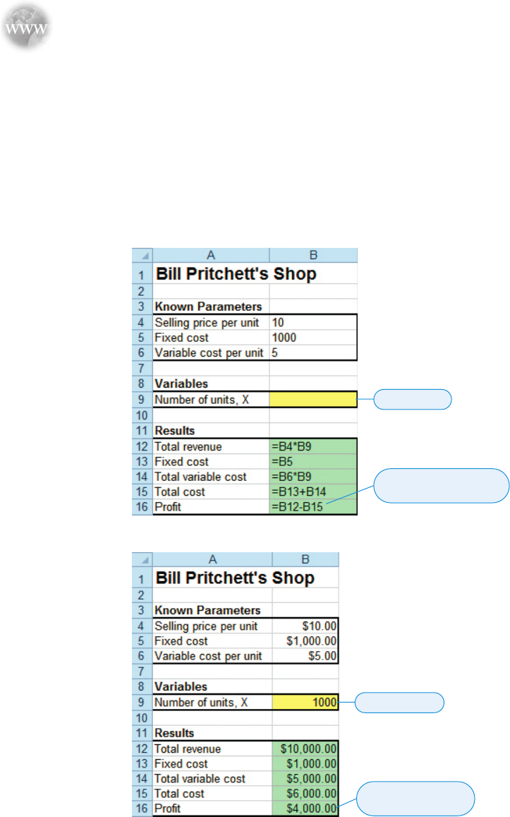
Screenshot 2A shows the formulas used in developing the decision model for Bill Pritchett’s

example. Cells B4, B5, and B6 show the known problem parameter values—namely, revenue

per unit, fixed cost, and variable cost per unit, respectively. Cell B9 is the lone variable in the

model, and it represents the number of units sold (i.e., X ). Using these entries, the total revenue,

total variable cost, total cost, and profit are computed in cells B12, B14, B15, and B16, respec-

tively. For example, if we enter a value of 1,000 units for X in cell B9, the profit is calculated as

$4,000 in cell B16, as shown in Screenshot 2B .

In addition to computing the profit, decision makers are often interested in the break-even

point (BEP) . The BEP is the number of units sold that will result in total revenue equaling total

costs (i.e., profit is $0). We can determine the BEP analytically by setting profit equal to $0 and

solving for X in Bill Pritchett’s profit expression. That is

File: 1-2.xls, sheets: 1-2A and 1-2B

The BEP results in $0 profit.

SCREENSHOT 2A

Formula View of Excel

Layout for Pritchett’s

Precious Time Pieces

Prot is revenue – xed

cost – variable cost.

Input variable

SCREENSHOT 2B

Excel Decision Model for

Pritchett’s Precious Time

Pieces

Prot is $4,000 if

1,000 units are sold.

1,000 units sold

INTRODUCTION TO MANAGERIAL DECISION MODELING

0  (Selling price per unit)  (Number of units)  (Fixed cost)

 (Variable cost per unit)  (Number of units)

which can be mathematically rewritten as

Break even point (BEP)  Fixed cost ⁄ (Selling price per unit

 Variable cost per unit) (2)

For Bill Pritchett’s example, we can compute the BEP as $1,000/($10 − $5) = 200 springs.

The BEP in dollars (which we denote as BEP

) can then be computed as

B E P

 Fixed cost  Variable costs  BEP (3)

For Bill Pritchett’s example, we can compute BEP

as $1,000 + $5 × 200 = $2,000.

Using Goal Seek to Find the Break-Even Point

While the preceding analytical computations for BEP and BEP

are fairly simple, an advantage

of using computer-based models is that many of these results can be calculated automatically.

For example, we can use a procedure in Excel called Goal Seek to calculate the BEP and BEP

values in the decision model shown in Screenshot 2B . The Goal Seek procedure allows us to

specify a desired value for a target cell . This target cell should contain a formula that involves a

different cell, called the changing cell . Once we specify the target cell, its desired value, and the

changing cell in Goal Seek , the procedure automatically manipulates the changing cell value to

try and make the target cell achieve its desired value.

In our case, we want to manipulate the value of the number of units X (in cell B9 of Screen-

shot 2B ) such that the profit (in cell B16 of Screenshot 2B ) takes on a value of zero. That is, cell

B16 is the target cell, its desired value is zero, and cell B9 is the changing cell. Observe that the

formula of profit in cell B16 is a function of the value of X in cell B9 (see Screenshot 2A ).

Screenshot 2C shows how the

Goal Seek procedure is implemented in Excel. As shown

in Screenshot 2C (a), we invoke Goal Seek by clicking the Data tab on Excel’s main menu bar,

followed by the What-If Analysis button (found in the Data Tools group within the Data tab),

and then finally on Goal Seek . The window shown in Screenshot 2C (b) is displayed. We specify

cell B16 in the Set cell box, a desired value of zero for this cell in the To value box, and cell B9

in the By changing cell box. When we now click OK , the Goal Seek Status window shown in

Screenshot 2C (c) is displayed, indicating that the target of $0 profit has been achieved. Cell B9

shows the resulting BEP value of 200 units. The corresponding BEP

value of $2,000 is shown

in cell B15.

Observe that we can use Goal Seek to compute the sales level needed to obtain any

desired profit. For example, see if you can verify that in order to get a profit of $10,000, Bill

Pritchett would have to sell 2,200 springs.

Excel’s Goal Seek can be used to

automatically find the BEP.

File: 1-2.xls, sheet: 1-2C

To provide meaningful assistance to Merrill Lynch, the man-

agement science group has concentrated on mathematical

models that focus on client satisfaction. What are the keys to

continued success for the management science group? Although

skill and technical expertise in decision modeling are essential,

the management science group has identified the following four

critical success factors: (1) objective analysis, (2) focus on busi-

ness impact and implementation, (3) teamwork, and (4) adopting

a disciplined consultative approach.

Source: From R. Nigam et al. “Bullish on Management Science,” OR/MS

Today, Vol. 27, No. 3 (June 2000): 48-51. Reprinted with permission.

Management science groups at corporations can make a

huge difference in reducing costs and increasing profits. At Merrill

Lynch, the management science group was established in 1986.

Its overall mission is to provide high-quality quantitative (or math-

ematical) analysis, modeling, and decision support. The group

analyzes a variety of problems and opportunities related to client

services, products, and the marketplace. In the past, this group

has helped Merrill Lynch develop asset allocation models, mutual

fund portfolio optimization solutions, investment strategy devel-

opment and research tools, financial planning models, and cross-

selling approaches.

IN ACTION

The Management Science Group Is

Bullish at Merrill Lynch

INTRODUCTION TO MANAGERIAL DECISION MODELING

Goal Seek

result window

Cell denoting prot.

Set prot to 0.

BEP is 200 units.

BEP

is $2,000.

Cell denoting number of units.

Prot target of $0

has been achieved.

(a)

(b)

(c)

Data tab in Excel

Goal Seek is part of What-If

Analysis in the Data Tools group.

SCREENSHOT 2C

Using Excel’s Goal Seek

to Compute the Break-

Even Point for Pritchett’s

Precious Time Pieces

6 Possible Problems in Developing Decision Models

We present the decision modeling approach as a logical and systematic means of tackling

decision-making problems. Even when these steps are followed carefully, however, many dif-

ficulties can hurt the chances of implementing solutions to real-world problems. We now look

at problems that can occur during each of the steps of the decision modeling approach.

Defining the Problem

In the worlds of business, government, and education, problems are, unfortunately, not easily

identified. Decision analysts typically face four roadblocks in defining a problem. We use an

application, inventory analysis, throughout this section as an example.

CONFLICTING VIEWPOINTS Analysts may often have to consider conflicting viewpoints in

defining a problem. For example, in inventory problems, financial managers usually feel that

inventory is too high because inventory represents cash not available for other investments. In

contrast, sales managers often feel that inventory is too low because high levels of inventory

may be needed to fill unexpected orders. If analysts adopt either of these views as the problem

definition, they have essentially accepted one manager’s perception. They can, therefore, expect

resistance from the other manager when the “solution” emerges. So it’s important to consider

both points of view before stating the problem.

Real-world problems are not

easily identifiable.

The problem needs to be

examined from several

viewpoints.

INTRODUCTION TO MANAGERIAL DECISION MODELING

IMPACT ON OTHER DEPARTMENTS Problems do not exist in isolation and are not owned by

just one department of a firm. For example, inventory is closely tied with cash flows and various

production problems. A change in ordering policy can affect cash flows and upset production

schedules to the point that savings on inventory are exceeded by increased financial and

production costs. The problem statement should therefore be as broad as possible and include

inputs from all concerned departments.

BEGINNING ASSUMPTIONS People often have a tendency to state problems in terms of

solutions. For example, the statement that inventory is too low implies a solution: that its

levels should be raised. An analyst who starts off with this assumption will likely find that

inventory should be raised! From an implementation perspective, a “good” solution to the

right problem is much better than an “optimal” solution to the wrong problem.

SOLUTION OUTDATED Even if a problem has been specified correctly at present, it can change

during the development of the model. In today’s rapidly changing business environment,

especially with the amazing pace of technological advances, it is not unusual for problems to

change virtually overnight. The analyst who presents solutions to problems that no longer exist

can’t expect credit for providing timely help.

Developing a Model

Even with a well-defined problem statement, a decision analyst may have to overcome hurdles

while developing decision models for real-world situations. Some of these hurdles are discussed

in the following sections.

FITTING THE TEXTBOOK MODELS A manager’s perception of a problem does not always

match the textbook approach. For example, most textbook inventory models involve minimizing

the sum of holding and ordering costs. Some managers view these costs as unimportant; instead,

they see the problem in terms of cash flow, turnover, and levels of customer satisfaction. The

results of a model based on holding and ordering costs are probably not acceptable to such

managers.

UNDERSTANDING A MODEL Most managers simply do not use the results of a model they

do not understand. Complex problems, though, require complex models. One trade-off is to

simplify assumptions in order to make a model easier to understand. The model loses some

of its reality but gains some management acceptance. For example, a popular simplifying

assumption in inventory modeling is that demand is known and constant. This allows analysts

to build simple, easy-to-understand models. Demand, however, is rarely known and constant, so

these models lack some reality. Introducing probability distributions provides more realism but

may put comprehension beyond all but the most mathematically sophisticated managers. In such

cases, one approach is for the decision analyst to start with the simple model and make sure that

it is completely understood. More complex models can then be introduced slowly as managers

gain more confidence in using these models.

Acquiring Input Data

Gathering the data to be used in the decision modeling approach to problem solving is often not

a simple task. Often, the data are buried in several different databases and documents, making it

very difficult for a decision analyst to gain access to the data.

USING ACCOUNTING DATA One problem is that most data generated in a firm come from

basic accounting reports. The accounting department collects its inventory data, for example, in

terms of cash flows and turnover. But decision analysts tackling an inventory problem need to

collect data on holding costs and ordering costs. If they ask for such data, they may be shocked

to find that the data were simply never collected for those specified costs.

Professor Gene Woolsey tells a story of a young decision analyst sent down to accounting

to get “the inventory holding cost per item per day for part 23456/AZ.” The accountant asked

the young man if he wanted the first-in, first-out figure; the last-in, first-out figure; the lower of

cost or market figure; or the “how-we-do-it” figure. The young man replied that the inventory

model required only one number. The accountant at the next desk said, “Heck, Joe, give the kid

a number.” The analyst was given a number and departed.

All inputs must be considered.

Managers do not use the

results of a model they do not

understand.

INTRODUCTION TO MANAGERIAL DECISION MODELING

VALIDITY OF DATA A lack of “good, clean data” means that whatever data are available

must often be distilled and manipulated (we call it “fudging”) before being used in a model.

Unfortunately, the validity of the results of a model is no better than the validity of the data that

go into the model. You cannot blame a manager for resisting a model’s “scientific” results when

he or she knows that questionable data were used as input.

Developing a Solution

An analyst may have to face two potential pitfalls while developing solutions to a decision

model. These are discussed in the following sections.

HARD-TO-UNDERSTAND MATHEMATICS The first concern in developing solutions is that

although the mathematical models we use may be complex and powerful, they may not be

completely understood. The aura of mathematics often causes managers to remain silent when

they should be critical. The well-known management scientist C. W. Churchman once cautioned

that “because mathematics has been so revered a discipline in recent years, it tends to lull the

unsuspecting into believing that he who thinks elaborately thinks well.”

THE LIMITATION OF ONLY ONE ANSWER The second problem in developing a solution is that

decision models usually give just one answer to a problem. Most managers would like to have

a range of options and not be put in a take-it-or-leave-it position. A more appropriate strategy

is for an analyst to present a range of options, indicating the effect that each solution has on the

objective function. This gives managers a choice as well as information on how much it will

cost to deviate from the optimal solution. It also allows problems to be viewed from a broader

perspective because it means that qualitative factors can also be considered.

Testing the Solution

The results of decision modeling often take the form of predictions of how things will work in

the future if certain changes are made in the present. To get a preview of how well solutions will

really work, managers are often asked how good a solution looks to them. The problem is that

complex models tend to give solutions that are not intuitively obvious. And such solutions tend to

be rejected by managers. Then a decision analyst must work through the model and the assump-

tions with the manager in an effort to convince the manager of the validity of the results. In the

process of convincing the manager, the analyst has to review every assumption that went into the

model. If there are errors, they may be revealed during this review. In addition, the manager casts

a critical eye on everything that went into the model, and if he or she can be convinced that the

model is valid, there is a good chance that the solution results are also valid.

Analyzing the Results

Once a solution has been tested, the results must be analyzed in terms of how they will affect the

total organization. You should be aware that even small changes in organizations are often diffi-

cult to bring about. If results suggest large changes in organizational policy, the decision analyst

can expect resistance. In analyzing the results, the analyst should ascertain who must change and

by how much, if the people who must change will be better or worse off, and who has the power

to direct the change.

The results of a model are only as

good as the input data used.

Hard-to-understand mathematics

and having only one answer

can be problems in developing

a solution.

Assumptions should be reviewed.

Churchman, C. W. “Reliability of Models in the Social Sciences,” Interfaces 4, 1 (November 1973): 1–12.

7 Implementation—Not Just the Final Step

We have just presented some of the many problems that can affect the ultimate acceptance of

decision modeling in practice. It should be clear now that implementation isn’t just another

step that takes place after the modeling process is over. Each of these steps greatly affects the

chances of implementing the results of a decision model.

Even though many business decisions can be made intuitively, based on hunches and

experience, there are more and more situations in which decision models can assist. Some

managers, however, fear that the use of a formal analytical process will reduce their

INTRODUCTION TO MANAGERIAL DECISION MODELING

decision-making power. Others fear that it may expose some previous intuitive decisions as

inadequate. Still others feel uncomfortable about having to reverse their thinking patterns with

formal decision making. These managers often argue against the use of decision modeling.

Many action-oriented managers do not like the lengthy formal decision-making process and

prefer to get things done quickly. They prefer “quick and dirty” techniques that can yield imme-

diate results. However, once managers see some quick results that have a substantial payoff, the

stage is set for convincing them that decision modeling is a beneficial tool.

We have known for some time that management support and user involvement are critical to

the successful implementation of decision modeling processes. A Swedish study found that only

40% of projects suggested by decision analysts were ever implemented. But 70% of the modeling

projects initiated by users, and fully 98% of projects suggested by top managers, were implemented.

Management support and user

involvement are important.

Summary

Decision modeling is a scientific approach to decision mak-

ing in practical situations faced by managers. Decision mod-

els can be broadly classified into two categories, based on

the type and nature of the problem environment under con-

sideration: (1) deterministic models and (2) probabilistic

models. Deterministic models assume that all the relevant

input data and parameters are known with certainty. In con-

trast, probabilistic models assume that some input data are

not known with certainty. The decision modeling approach

includes three major steps: (1) formulation, (2) solution, and

(3) interpretation. It is important to note that it is common

to iterate between these three steps before the final solution

is obtained. Spreadsheets are commonly used to develop

decision models.

In using the decision modeling approach, however, there

can be potential problems, such as conflicting viewpoints,

disregard of the impact of the model on other departments,

outdated solutions, misunderstanding of the model, difficulty

acquiring good input data, and hard-to-understand mathemat-

ics. In using decision models, implementation is not the final

step. There can be a lack of commitment to the approach and

resistance to change.

Glossary

Break-Even Point (BEP) The number of units sold that

will result in total revenue equaling total costs (i.e., profit

is $0).

Break-Even Point in Dollars (BEP

) The sum of fixed and

total variable cost if the number of units sold equals the

break-even point.

Decision Analyst An individual who is responsible for

developing a decision model.

Decision Modeling A scientific approach that uses quantitative

(mathematical) techniques as a tool in managerial decision

making. Also known as quantitative analysis , management

science , and operations research .

Deterministic Model A model which assumes that all the

relevant input data and parameters are known with certainty.

Formulation The process by which each aspect of a prob-

lem scenario is translated and expressed in terms of a

mathematical model.

Goal Seek A feature in Excel that allows users to specify a

goal or target for a specific cell and automatically manipu-

late another cell to achieve that target.

Input Data Data that are used in a model in arriving at the

final solution.

Model A representation (usually mathematical) of a practical

problem scenario or environment.

Probabilistic Model A model which assumes that some input

data are not known with certainty.

Problem Parameter A measurable quantity that is inherent

in a problem. It typically has a fixed and known value (i.e.,

a constant).

Sensitivity Analysis A process that involves determining

how sensitive a solution is to changes in the formulation

of a problem.

Variable A measurable quantity that may vary or that is sub-

ject to change.

Discussion Questions and Problems

Discussion Questions

1 Define decision modeling . What are some of the organi-

zations that support the use of the scientific approach?

2 What is the difference between deterministic and

probabilistic models? Give several examples of each

type of model.

3 What are the differences between quantitative and qualita-

tive factors that may be present in a decision model?

4 Why might it be difficult to quantify some qualitative

factors in developing decision models?

5 What steps are involved in the decision modeling

process? Give several examples of this process.

INTRODUCTION TO MANAGERIAL DECISION MODELING

6 Why is it important to have an iterative process

between the steps of the decision modeling approach?

7 Briefly trace the history of decision modeling. What

happened to the development of decision modeling

during World War II?

8 What different types of models are mentioned in this

chapter? Give examples of each.

9 List some sources of input data.

10 Define decision variable . Give some examples of

variables in a decision model.

11 What is a problem parameter? Give some examples

of parameters in a decision model.

12 List some advantages of using spreadsheets for deci-

sion modeling.

13 What is implementation, and why is it important?

14 Describe the use of sensitivity analysis, or postopti-

mality analysis, in analyzing the results of decision

models.

15 Managers are quick to claim that decision modelers

talk to them in a jargon that does not sound like Eng-

lish. List four terms that might not be understood by

a manager. Then explain in nontechnical terms what

each of them means.

16 Why do you think many decision analysts don’t like

to participate in the implementation process? What

could be done to change this attitude?

17 Should people who will be using the results of a new

modeling approach become involved in the techni-

cal aspects of the problem-solving procedure?

18 C. W. Churchman once said that “mathematics tends

to lull the unsuspecting into believing that he who

thinks elaborately thinks well.” Do you think that

the best decision models are the ones that are most

elaborate and complex mathematically? Why?

Problems

19 A Website has a fixed cost $15,000 per day. The

revenue is $0.06 each time the Website is accessed.

The variable cost of responding to each hit is $0.02.

(a) How many times must this Website be accessed

each day to break even?

(b) What is the break-even point, in dollars?

20 An electronics firm is currently manufacturing

an item that has a variable cost of $0.60 per unit

and selling price of $1.10 per unit. Fixed costs are

$15,500. Current volume is 32,000 units. The firm

can substantially improve the product quality by

adding a new piece of equipment at an additional

fixed cost of $8,000. Variable cost would increase

to $0.70, but volume is expected to jump to 50,000

units due to the higher quality of the product.

(a) Should the company buy the new equipment?

(b) Compute the profit with the current equipment

and the expected profit with the new equipment.

21 A manufacturer is evaluating options regarding

his production equipment. He is trying to decide

whether he should refurbish his old equipment for

$70,000, make major modifications to the produc-

tion line for $135,000, or purchase new equipment

for $230,000. The product sells for $10, but the

variable costs to make the product are expected to

vary widely, depending on the decision that is to

be made regarding the equipment. If the manufac-

turer refurbishes, the variable costs will be $7.20 per

unit. If he modifies or purchases new equipment, the

variable costs are expected to be $5.25 and $4.75,

respectively.

(a) Which alternative should the manufacturer

choose if it the demand is expected to be between

30,000 and 40,000 units?

(b) What will be the manufacturer’s profit if the

demand is 38,000 units?

22 St. Joseph’s School has 1,200 students, each of

whom currently pays $8,000 per year to attend. In

addition to revenues from tuition, the school receives

an appropriation from the church to sustain its activ-

ity. The budget for the upcoming year is $15 million,

and the church appropriation will be $4.8 million.

By how much will the school have to raise tuition

per student to keep from having a shortfall in the

upcoming year?

23 Refer to Problem 22. Sensing resistance to the idea

of raising tuition from members of St. Joseph’s

Church, one of the board members suggested that

the 960 children of church members could pay

$8,000 as usual. Children of nonmembers would pay

more. What would the nonmember tuition per year

be if St. Joseph’s wanted to continue to plan for a

$15 million budget?

24 Refer to Problems 22 and 23. Another board mem-

ber believes that if church members pay $8,000 in

tuition, the most St. Joseph’s can increase nonmem-

ber tuition is $1,000 per year. She suggests that an-

other solution might be to cap nonmember tuition

at $9,000 and attempt to recruit more nonmember

students to make up the shortfall. Under this plan,

how many new nonmember students will need to be

recruited?

25 Great Lakes Automotive is considering producing,

in-house, a gear assembly that it currently purchases

from Delta Supply for $6 per unit. Great Lakes esti-

mates that if it chooses to manufacture the gear as-

sembly, it will cost $23,000 to set up the process and

then $3.82 per unit for labor and materials. At what

volume would these options cost Great Lakes the

same amount of money?

26 A start-up publishing company estimates that the

fixed costs of its first major project will be $190,000,

the variable cost will be $18, and the selling price

per book will be $34.

INTRODUCTION TO MANAGERIAL DECISION MODELING

19 (a) 375,000. (b) $22,500.

21 (a) Make major modifications. (b) $45,500.

23 $10,500.

25 10,550 units.

27 Yes. The profit will increase by $1,000.

29 (a) BEP

= 6,250. BEP

= 7,750. (b) Choose A.

this production level.

(a) How many books must be sold for this project to

break even?

(b) Suppose the publishers wish to take a total of

$40,000 in salary for this project. How many

books must be sold to break even, and what is

the break-even point, in dollars?

27 The electronics firm in Problem 20 is now consid-

ering purchasing the new equipment and increas-

ing the selling price of its product to $1.20 per

unit. Even with the price increase, the new volume

is expected to be 50,000 units. Under these cir-

cumstances, should the company purchase the new

equipment and increase the selling price?

28 A distributer of prewashed shredded lettuce is

opening a new plant and considering whether to

use a mechanized process or a manual process to

prepare the product. The manual process will have

a fixed cost of $43,400 per month and a variable

cost of $1.80 per 5-pound bag. The mechanized

process would have a fixed cost of $84,600 per

month and a variable cost of $1.30 per bag. The

company expects to sell each bag of shredded let-

tuce for $2.50.

(a) Find the break-even point for each process.

(b) What is the monthly profit or loss if the company

chooses the manual process and sells 70,000

bags per month?

29 A fabrication company must replace its widget

machine and is evaluating the capabilities of two avail-

able machines. Machine A would cost the company

$75,000 in fixed costs for the first year. Each widget

produced using Machine A would have a variable cost

of $16. Machine B would have a first-year fixed cost

of $62,000, and widgets made on this machine would

have a variable cost of $20. Machine A would have

the capacity to make 18,000 widgets per year, which is

approximately double the capacity for Machine B.

(a) If widgets sell for $28 each, find the break-even

point for each machine. Consider first-year costs

only.

(b) If the fabrication company estimates a demand

of 6,500 units in the next year, which machine

should be selected?

tion machines cost the same?

30 Bismarck Manufacturing intends to increase capac-

ity through the addition of new equipment. Two

vendors have presented proposals. The fixed cost for

proposal A is $65,000, and for proposal B, $34,000.

The variable cost for A is $10, and for B, $14. The

revenue generated by each unit is $18.

(a) What is the break-even point for each proposal?

(b) If the expected volume is 8,300 units, which

alternative should be chosen?

Brief Solutions to Odd-Numbered End-of-Chapter Problems

1 Introduction

2 Developing a Linear Programming Model

3 Formulating a Linear Programming Problem

4 Graphical Solution of a Linear Programming

Problem with Two Variables

5 A Minimization Linear Programming Problem

6 Special Situations in Solving Linear Programming

Problems

7 Setting Up and Solving Linear Programming

Problems Using Excel’s Solver

8 Algorithmic Solution Procedures for Linear

Programming Problems

After completing this chapter, students will be able to:

1. Understand the basic assumptions and properties

of linear programming (LP).

2. Use graphical procedures to solve LP problems

with only two variables to understand how LP

problems are solved.

3. Understand special situations such as

redundancy, infeasibility, unboundedness, and

alternate optimal solutions in LP problems.

4. Understand how to set up LP problems on a

spreadsheet and solve them using Excel’s Solver.

CHAPTER OUTLINE

Summary • Glossary • Solved Problems • Discussion Questions and Problems • Case Study: Mexicana Wire

Winding, Inc. • Case Study: Golding Landscaping and Plants, Inc. • Internet Case Studies

LEARNING OBJECTIVES

Linear Programming

Models: Graphical and

Computer Methods

The companion website for this text is www.pearsonhighered.com/balakrishnan.

From Chapter 2 of Managerial Decision Modeling with Spreadsheets, Third Edition. Nagraj Balakrishnan, Barry Render, Ralph M. Stair, Jr.

LINEAR PROGRAMMING MODELS: GRAPHICAL AND COMPUTER METHODS

Management decisions in many organizations involve trying to make the most effective use of

resources. Resources typically include machinery, labor, money, time, warehouse space, and

raw materials. These resources can be used to manufacture products (e.g., computers, automo-

biles, furniture, clothing) or provide services (e.g., package delivery, health services, advertising

policies, investment decisions).

In all resource allocation situations, the manager must sift through several thousand decision

choices or alternatives to identify the best, or optimal, choice. The most widely used decision

modeling technique designed to help managers in this process is called mathematical program-

ming . The term mathematical programming is somewhat misleading because this modeling

technique requires no advanced mathematical ability (it uses just basic algebra) and has nothing

whatsoever to do with computer software programming! In the world of decision modeling,

programming refers to setting up and solving a problem mathematically.

Within the broad topic of mathematical programming, the most widely used modeling tech-

nique designed to help managers in planning and decision making is linear programming (LP) .

When developing LP (and other mathematical programming)–based decision models, we

assume that all the relevant input data and parameters are known with certainty. For this reason,

these types of decision modeling techniques are classified as deterministic models.

Computers have, of course, played an important role in the advancement and use of LP.

Real-world LP problems are too cumbersome to solve by hand or with a calculator, and com-

puters have become an integral part of setting up and solving LP models in today’s business

environments. Over the past decade, spreadsheet packages such as Microsoft Excel have be-

come increasingly capable of handling many of the decision modeling techniques (including

LP and other mathematical programming models) that are commonly encountered in practical

situations.

Linear programming helps in

resource allocation decisions.

We focus on using Excel to set

up and solve LP models.

L inear programming was conceptually developed before World

War II by the outstanding Soviet mathematician A. N. Kolmogorov.

Another Russian, Leonid Kantorovich, won the Nobel Prize in Eco-

nomics for advancing the concepts of optimal planning. An early

application of linear programming, by George Stigler in 1945,

was in the area we today call “diet problems.”

Major progress in the field, however, took place in 1947 and

later, when George D. Dantzig developed the solution procedure

known as the simplex algorithm. Dantzig, then a U.S. Air Force

mathematician, was assigned to work on logistics problems.

He noticed that many problems involving limited resources and

more than one demand could be set up in terms of a series of

equations and inequalities. Although early LP applications were

military in nature, industrial applications rapidly became appar-

ent with the spread of business computers. In 1984, Narendra

Karmarkar developed an algorithm that appears to be superior to

the simplex method for many very large applications.

HISTORY

How Linear Programming Started

1 Introduction

2 Developing a Linear Programming Model

Since the mid-twentieth century, LP has been applied extensively to medical, transportation,

operations, financial, marketing, accounting, human resources, and agricultural problems.

Regardless of the size and complexity of the decision-making problem at hand in these diverse

applications, the development of all LP models can be viewed in terms of the three distinct

steps: (1) formulation, (2) solution, and (3) interpretation. We now discuss each with regard to

LP models.

LINEAR PROGRAMMING MODELS: GRAPHICAL AND COMPUTER METHODS

Formulation

Formulation is the process by which each aspect of a problem scenario is translated and

expressed in terms of simple mathematical expressions. The aim in LP formulation is to ensure

that the set of mathematical equations, taken together, completely addresses all the issues relevant

to the problem situation at hand. We demonstrate a few examples of simple LP formulations in

this chapter.

Solution

The solution step is where the mathematical expressions resulting from the formulation pro-

cess are solved to identify an optimal (or best) solution to the model.

In this text, the focus is

on solving LP models using spreadsheets. However, we briefly discuss graphical solution pro-

cedures for LP models involving only two variables. The graphical solution procedure is useful

in that it allows us to provide an intuitive explanation of the procedure used by most software

packages to solve LP problems of any size.

Interpretation and Sensitivity Analysis

Assuming that a formulation is correct and has been successfully implemented and solved using

an LP software package, how does a manager use the results? In addition to just providing the

solution to the current LP problem, the computer results also allow the manager to evaluate the

impact of several different types of what-if questions regarding the problem.

In this text, our emphasis is on formulation and interpretation, along with detailed descrip-

tions of how spreadsheets can be used to efficiently set up and solve LP models.

Properties of a Linear Programming Model

All LP models have the following properties in common:

1. All problems seek to maximize or minimize some quantity, usually profit or cost. We refer

to this property as the objective function of an LP problem. For example, the objective of

a typical manufacturer is to maximize profits. In the case of a trucking or railroad distribu-

tion system, the objective might be to minimize shipping costs. In any event, this objective

must be stated clearly and defined mathematically. It does not matter whether profits and

cost are measured in cents, dollars, euros, or millions of dollars. An optimal solution to the

problem is the solution that achieves the best value (maximum or minimum, depending on

the problem) for the objective function.

2. LP models usually include restrictions, or constraints , that limit the degree to which we

can pursue our objective. For example, when we are trying to decide how many units to

produce of each product in a firm’s product line, we are restricted by the available machin-

ery time. Likewise, in selecting food items for a hospital meal, a dietitian must ensure that

minimum daily requirements of vitamins, protein, and so on are satisfied. We want, there-

fore, to maximize or minimize a quantity (the objective) subject to limited resources (the

constraints).

An LP model usually includes a set of constraints known as nonnegativity constraints .

These constraints ensure that the variables in the model take on only nonnegative values

(i.e., Ú 0 ). This is logical because negative values of physical quantities are impossible;

you simply cannot produce a negative number of chairs or computers.

3. There must be alternative courses of action from which we can choose. For example, if a

company produces three different products, management could use LP to decide how to

allocate its limited production resources (of personnel, machinery, and so on) among these

products. Should it devote all manufacturing capacity to make only the first product, should

it produce equal numbers or amounts of each product, or should it allocate the resources in

some other ratio? If there were no alternative to select from, we would not need LP.

Formulation involves expressing

a problem scenario in terms of

simple mathematical expressions.

Solution involves solving

mathematical expressions to find

values for the variables.

Sensitivity analysis allows a

manager to answer “what-if”

questions regarding a problem’s

solution.

First LP property: Problems seek

to maximize or minimize an

objective.

Second LP property: Constraints

limit the degree to which the

objective can be obtained.

Third LP property: There must be

alternatives available.

We refer to the best solution as

have more than one optimal solution.

an optimal solution rather than as the optimal solution because the problem could

LINEAR PROGRAMMING MODELS: GRAPHICAL AND COMPUTER METHODS

4. The objective and constraints in LP problems must be expressed in terms of linear equa-

tions or inequalities. In linear mathematical relationships, all terms used in the objective

function and constraints are of the first degree (i.e., not squared, or to the third or higher

power, or appearing more than once). Hence, the equation 2A + 5B = 10 is a valid

linear function, whereas the equation 2A

+ 5B

+ AB = 10 is not linear because the

variable A is squared, the variable B is cubed, and the two variables appear as a product in

the third term.

You will see the term inequality quite often when we discuss LP problems. By inequality

we mean that not all LP constraints need be of the form A + B = C. This particular relation-

ship, called an equation, implies that the sum of term A and term B exactly equals term C . In

most LP problems, we see inequalities of the form A + B … C o r A + B Ú C. The first of

these means that A plus B is less than or equal to C . The second means that A plus B is greater

than or equal to C . This concept provides a lot of flexibility in defining problem limitations.

Basic Assumptions of a Linear Programming Model

Technically, there are four additional requirements of an LP problem of which you should be

aware:

1. We assume that conditions of certainty exist. That is, numbers used in the objective func-

tion and constraints are known with certainty and do not change during the period being

studied.

2. We also assume that proportionality exists in the objective function and constraints. This

means that if production of 1 unit of a product uses 3 hours of a particular resource, then

making 10 units of that product uses 30 hours of the resource.

3. The third assumption deals with additivity , meaning that the total of all activities equals the

sum of the individual activities. For example, if an objective is to maximize profit = $8

per unit of the first product made plus $3 per unit of the second product made, and if 1 unit

of each product is actually produced, the profit contributions of $8 and $3 must add up to

produce a sum of $11.

4. We make the divisibility assumption that solutions need not necessarily be in whole num-

bers (integers). That is, they may take any fractional value. If a fraction of a product cannot

be produced (e.g., one-third of a submarine), an integer programming problem exists.

Fourth LP property:

Mathematical relationships

are linear.

An inequality has a … or Ú sign.

Four technical requirements

are certainty, proportionality,

additivity, and divisibility.

Technically, we maximize total contribution margin, which is the difference between unit selling price and costs

that vary in proportion to the quantity of the item produced. Depreciation, fixed general expense, and advertising are

excluded from calculations.

3 Formulating a Linear Programming Problem

One of the most common LP applications is the product mix problem . In many manufactur-

ing firms, two or more products are usually produced using limited resources, such a personnel,

machines, raw materials, and so on. The profit that the firm seeks to maximize is based on the

profit contribution per unit of each product. (Profit contribution, is the selling price per unit minus

the variable cost per unit.

) The firm would like to determine how many units of each product it

should produce so as to maximize overall profit, given its limited resources.

We begin our discussion of LP formulation with a simple product mix problem that involves

only two variables (one for each product, in this case). We recognize that in most real-world

situations, there is very little chance we will encounter LP models with just two variables. Such

LP models therefore have little real-world value. We nevertheless consider it worthwhile to

study these models here for two reasons. First, the compact size of these models makes it easier

for a beginning student to understand the structure of LP models and the logic behind their

formulation. The same structure and logic carry forward even to problems of larger size. Sec-

ond, and more importantly, as we will see in section 4, we can represent a two-variable model

in a graphical form, which allows us to visualize the interaction between various issues in the

problem.

Product mix problems use LP

to decide how much of each

product to make, given a series of

resource restrictions.

Problems with only two variables

are uncommon in practice.

LINEAR PROGRAMMING MODELS: GRAPHICAL AND COMPUTER METHODS

Linear Programming Example: Flair Furniture Company

Flair Furniture Company produces inexpensive tables and chairs. The production process for

each is similar in that both require a certain number of labor hours in the carpentry department

and a certain number of labor hours in the painting department. Each table takes 3 hours of car-

pentry work and 2 hours of painting work. Each chair requires 4 hours of carpentry and 1 hour

of painting. During the current month, 2,400 hours of carpentry time and 1,000 hours of painting

time are available. The marketing department wants Flair to make no more than 450 new chairs

this month because there is a sizable existing inventory of chairs. However, because the existing

inventory of tables is low, the marketing department wants Flair to make at least 100 tables this

month. Each table sold results in a profit contribution of $7, and each chair sold yields a profit

contribution of $5.

Flair Furniture’s problem is to determine the best possible combination of tables and chairs

to manufacture this month in order to attain the maximum profit. The firm would like this prod-

uct mix situation formulated (and subsequently solved) as an LP problem.

To provide a structured approach for formulating this problem (and any other LP problem,

irrespective of size and complexity), we present a three-step process in the following sections.

Decision Variables

Decision variables (or choice variables) represent the unknown entities in a problem—that is,

what we are solving for in the problem. For example, in the Flair Furniture problem, there are

two unknown entities: the number of tables to be produced this month and the number of chairs

to be produced this month. Note that all other unknowns in the problem (e.g., the total carpentry

time needed this month) can be expressed as linear functions of the number of tables produced

and the number of chairs produced.

Decision variables are expressed in the problems using alphanumeric symbols. When writing

the formulation on paper, it is convenient to express the decision variables using simple names

that are easy to understand. For example, the number of tables to be produced can be denoted

by names such as T , Tables , or X

, and the number of chairs to be produced can be denoted by

names such as C , Chairs , or X

Throughout this text, to the extent possible, we use self-explanatory names to denote

the decision variables in our formulations. For example, in Flair Furniture’s problem, we use

T and C to denote the number of tables and chairs to be produced this month, respectively.

Although the two decision variables in Flair’s model define similar entities (in the sense

that they both represent the number of units of a product to make), this need not be the case in all

LP (and other) decision models. It is perfectly logical for different decision variables in the same

model to define completely different entities and be measured in different units. For example,

variable X can denote the amount of labor to use (measured in hours), while variable Y can

denote the amount of paint to use (measured in gallons).

The Objective Function

The objective function states the goal of a problem—that is, why we are trying to solve the prob-

lem. An LP model must have a single objective function. In most business-oriented LP models,

the objective is to either maximize profit or minimize cost. The goal in this step is to express the

profit (or cost) in terms of the decision variables defined earlier. In Flair Furniture’s problem,

the total profit can be expressed as

P r o f i t = 1+7

profit

per

table2* 1number

tables

produced2

+ 1+5

profit

per

chair2* 1number

chairs

produced2

Using the decision variables T and C defined earlier, the objective function can be written as

M a x i m i z e

+7T + +5C

Constraints

Constraints denote conditions that prevent us from selecting any value we please for the deci-

sion variables. An LP model can have as many constraints as necessary for a problem scenario.

Each constraint is expressed as a mathematical expression and can be independent of the other

constraints in the model.

Decision variables are the

unknown entities in a problem.

The problem is solved to find

values for decision variables.

Different decision variables in

the same model can be measured

in different units.

The objective function represents

the motivation for solving a

problem.

Constraints represent

restrictions on the values the

decision variables can take.

LINEAR PROGRAMMING MODELS: GRAPHICAL AND COMPUTER METHODS

In Flair’s problem, we note that there are four restrictions on the solution. The first two have to

do with the carpentry and painting times available. The third and fourth constraints deal with mar-

keting-specified production conditions on the numbers of chairs and tables to make, respectively.

With regard to the carpentry and painting times, the constraints must ensure that the amount

of the resource (time) required by the production plan is less than or equal to the amount of the

resource (time) available. For example, in the case of carpentry, the total time used is

hour

per

table2* 1number

tables

produced2

+ 14

hours

per

chair2* 1number

chairs

produced2

There are 2,400 hours of carpentry time available. Using the decision variables T and C defined

earlier, this constraint can be stated as

3 T + 4C … 2,400

Likewise, the second constraint specifies that the painting time used is less than or equal to

the painting time available. This can be stated as

2 T + 1C … 1,000

Next, there is the marketing-specified constraint that no more than 450 chairs be produced.

This can be expressed as

C … 450

Finally, there is the second marketing-specified constraint that at least 100 tables must be

produced. Note that unlike the first three constraints, this constraint involves the Ú sign because

100 is a minimum requirement. It is very common in practice for a single LP model to include

constraints with different signs (i.e., … ,

Ú , and = ). The constraint on the production of tables

can be expressed as

T Ú 100

All four constraints represent restrictions on the numbers that we can make of the two prod-

ucts and, of course, affect the total profit. For example, Flair cannot make 900 tables because

the carpentry and painting constraints are both violated if T = 900. Likewise, it cannot make

500 tables and 100 chairs, because that would require more than 1,000 hours of painting time.

Hence, we note one more important aspect of LP models: Certain interactions exist between

variables. The more units of one product that a firm produces, the fewer it can make of other

products. We show how this concept of interaction affects the solution to the model as we tackle

the graphical solution approach in the next section.

Nonnegativity Constraints and Integer Values

Before we consider the graphical solution procedure, there are two other issues we need to address.

First, because Flair cannot produce negative quantities of tables or chairs, the nonnegativity

constraints must be specified. Mathematically, these can be stated as

T Ú 0

1number

tables

produced Ú 02

C Ú 0

1number

chairs

produced Ú 02

Second, it is possible that the optimal solution to the LP model will result in fractional val-

ues for T and C . Because the production plan in Flair’s problem refers to a month’s schedule, we

can view fractional values as work-in-process inventory that is carried over to the next month.

However, in some problems, we may require the values for decision variables to be whole num-

bers (integers) in order for the solution to make practical sense. A model in which some or all of

the decision variables are restricted only to integer values is called an integer programming ( IP )

model. In general, it is considerably more difficult to solve an IP problem than an LP problem.

Further, LP model solutions allow detailed sensitivity analysis to be undertaken, whereas IP

model solutions do not. For these reasons, we do not specify the integer requirement in LP mod-

els, and we permit fractional values in the solution. Fractional values can then be rounded off

appropriately, if necessary.

The resource constraints put

limits on the carpentry time

and painting time needed

mathematically.

It is common for different

constraints to have different

signs in an LP model.

A key principle of LP is that

interactions exist between

variables.

Nonnegativity constraints specify

that decision variables cannot

have negative values.

In LP models, we do not specify

that decision variables should

only have integer values.

LINEAR PROGRAMMING MODELS: GRAPHICAL AND COMPUTER METHODS

Guidelines to Developing a Correct LP Model

We have now developed our first LP model. Before we proceed further, let us address a question

that many students have, especially at the early stages of their experience with LP formulation:

“How do I know my LP model is right?” There is, unfortunately, no simple magical answer for

this question. Instead, we offer the following guidelines that students can use to judge on their own

whether their model does what it is intended to do. Note that these guidelines do not guarantee that

your model is correct. Formulation is still an art that you master only through repeated application

to several diverse problems. However, by following these guidelines, you can hopefully avoid the

common errors that many beginners commit:



Recognizing and defining the decision variables is perhaps the most critical step in LP

formulation. In this endeavor, one approach we have often found useful and effective is

to assume that you have to communicate your result to someone else. When you tell that

person “The answer is to do —————,” what exactly do you need to know to fill in the

blank? Those entities are usually the decision variables.



Remember that it is perfectly logical for different decision variables in a single LP model

to be measured in different units. That is, all decision variables in an LP model need not

denote similar entities.



All expressions in the model (the objective function and each constraint) must use only

the decision variables that have been defined for the model. For example, in the Flair

Furniture problem, the decision variables are T and C . Notice that all expressions involve

only T and C . It is, of course, permissible for a decision variable to not be part of a specific

expression. For example, the variable T is not part of the constraint C … 450.



At any stage of the formulation, if you find yourself unable to write a specific expression

(the objective function or a constraint) using the defined decision variables, it is a pretty

good indication that you either need more decision variables or you’ve defined your

decision variables incorrectly.



All terms within the same expression must refer to the same entity. Consider, for example,

the expression for the carpentry constraint 3T + 4C … 2,400. Notice that each term

(i.e., 4 T , 3 C , and 2,400) measures an amount of carpentry time. Likewise, in the objective

function, each term (i.e., $7 T and $5 C ) in the expression measures profit.



All terms within the same expression must be measured in the same units. That is, if the

first term in an expression is in hours, all other terms in that expression must also be in

hours. For example, in the carpentry constraint 3T + 4C … 2,400, the 4T,

3C, and 2,400

are each measured in hours.



Address each constraint separately. That is, there is no single “mega” expression that will

take care of all constraints in the model at one time. Each constraint is a separate issue,

Here are a few guidelines to

developing a correct LP model.

General Electric Asset Management Incorporated (GEAM)

manages investment portfolios worth billions of dollars on behalf

of various General Electric (GE) units and other clients worldwide,

including Genworth Financial and GE Insurance (GEI). GEAM, a

wholly owned subsidiary of GE, invests portfolios of assets pri-

marily in corporate and government bonds, taking into account

risk and regulatory constraints. The objective is to identify the

portfolios’ risk/return trade-offs by maximizing the return or mini-

mizing the risk. While risk is widely represented by variance or

volatility, it is usually a nonlinear measure and portfolio managers

typically use linear risk sensitivities for computational tractability.

To address this problem, a multidisciplinary team from GE

Global Research Center worked with GEAM, Genworth, and

GEI to develop a sequential linear-programming algorithm that

handles the risk nonlinearity iteratively but efficiently. The team

determined that the optimal solution for the portfolio manage-

ment problem would result in improved financial performance

and better understanding of the risk/return trade-off. GE initially

used the algorithm on a limited basis to optimize portfolios val-

ued at over $30 billion. It is now in broader use at GEAM, GEI,

and Genworth. It is estimated that for every $100 billion of assets,

the present value of potential benefits is around $75 million over

five years.

Source: Based on K. C. Chalermkraivuth et al. “GE Asset Management,

Genworth Financial, and GE Insurance Use a Sequential-Linear-Programming

Algorithm to Optimize Portfolios,” Interfaces 35, 5 (September-October

2005): 370–380.

IN ACTION

Linear Programing Helps General Electric

Units to Optimize Portfolios

LINEAR PROGRAMMING MODELS: GRAPHICAL AND COMPUTER METHODS

and you must write a separate expression for each one. While writing one constraint

(e.g., carpentry time), do not worry about other constraints (e.g., painting time).



Try “translating” the mathematical expression back to words. After all, writing a constraint

is just a matter of taking a problem scenario that is in words (e.g., “the amount of the

carpentry time required by the production plan should be less than or equal to the carpen-

try time available”) and translating it to a simple linear mathematical expression (e.g.,

3 T + 4C … 2,400 ). To make sure the translation has been done correctly, do the reverse

process. That is, try explaining in words (to yourself) what the expression you have just

written is saying. While doing so, make sure you remember the previous guidelines about

all terms in an expression dealing with the same issue and being measured in the same

units. If your “reverse translation” yields exactly the situation that you were trying to

express in mathematical form, chances are your expression is correct.

4 Graphical Solution of a Linear Programming Problem with Two Variables

As noted earlier, there is little chance of encountering LP models with just two variables in real-

world situations. However, a major advantage of two-variable LP models (such as Flair Furni-

ture’s problem) is that they can be graphically illustrated using a two-dimensional graph. This

graph can then be used to identify the optimal solution to the model. Although this graphical so-

lution procedure has limited value in real-world situations, it is invaluable in two respects. First,

it provides insights into the properties of solutions to all LP models, regardless of their size.

Second, even though we use a computerized spreadsheet based procedure to solve LP models in

this text, the graphical procedure allows us to provide an intuitive explanation of how this more

complex solution procedure works for LP models of any size. For these reasons, we first discuss

the solution of Flair’s problem using a graphical approach.

Graphical Representation of Constraints

The complete LP model for Flair’s problem can be restated as follows:

M a x i m i z e

profit = +7T + +5C

subject to the constraints

3 T + 4C … 2,400

1carpentry

time2

2 T + 1C … 1,000

1painting

time2

C … 450

1maximum

chairs

allowed2

T Ú 100

1minimum

tables

required2

C Ú 0

1nonnegativity2

To find an optimal solution to this LP problem, we must first identify a set, or region, of feasible

solutions. The first step in doing so is to plot each of the problem’s constraints on a graph. We can

plot either decision variable on the horizontal ( X ) axis of the graph, and the other variable on the

vertical ( Y) axis. In Flair’s case, let us plot T (tables) on the X -axis and C (chairs) on the Y- axis.

The nonnegativity constraints imply that we are working only in the first (or positive) quadrant

of a graph.

CARPENTRY TIME CONSTRAINT To represent the carpentry constraint graphically, we first

convert the expression into a linear equation (i.e., 3T + 4C = 2,400 ) by replacing the inequality

sign 1…2 with an equality sign 1= 2.

As you may recall from elementary algebra, the solution of a linear equation with two vari-

ables represents a straight line. The easiest way to plot the line is to find any two points that

satisfy the equation and then draw a straight line through them. The two easiest points to find are

generally the points at which the line intersects the horizontal ( T ) and vertical ( C ) axes.

If Flair produces no tables (i.e., T = 0 ), then 3102+ 4C = 2,400, or C = 600. That is,

the line representing the carpentry time equation crosses the vertical axis at C = 600. This indi-

cates that if the entire carpentry time available is used to make only chairs, Flair could make

600 chairs this month.

The graphical method works

only when there are two decision

variables, but it provides valuable

insight into how larger problems

are solved.

Here is a complete mathematical

statement of the Flair LP

problem.

Nonnegativity constraints mean

we are always in the graphical

area where T Ú 0 and C Ú 0.

Plotting the first constraint

involves finding points at which

the line intersects the T -axis and

C -axis.

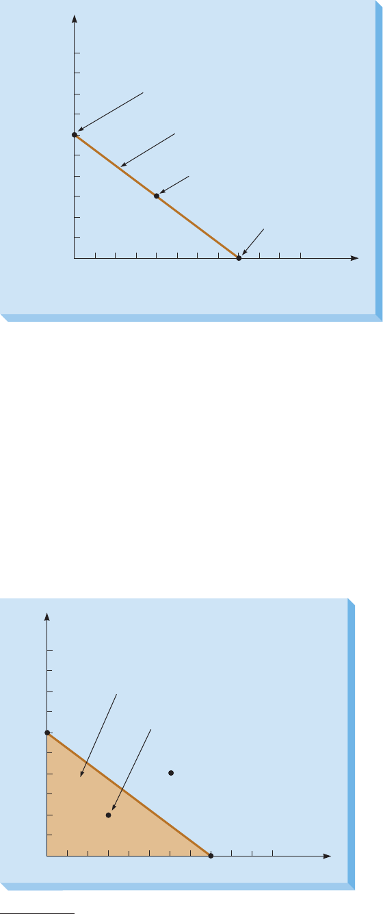
LINEAR PROGRAMMING MODELS: GRAPHICAL AND COMPUTER METHODS

To find the point at which the line 3T + 4C = 2,400 crosses the horizontal axis, let us

assume that Flair uses all the carpentry time available to make only tables. That is, C = 0. Then

3 T + 4102= 2,400, or T = 800.

The nonnegativity constraints and the carpentry constraint line are illustrated in Figure 1 .

The line running from point 1T = 0,

C = 6002 to point 1T = 800,

C = 02 represents the car-

pentry time equation 3T + 4C = 2,400. We know that any combination of tables and chairs

represented by points on this line (e.g., T = 400,

C = 300 ) will use up all 2,400 hours of

carpentry time.

Recall, however, that the actual carpentry constraint is the inequality 3T + 4C … 2,400.

How do we identify all the points on the graph that satisfy this inequality? To do so, we check

any possible point in the graph. For example, let us check 1T = 300,

C = 2002. If we substitute

these values in the carpentry constraint, the result is 3 * 300 + 4 * 200 = 1,700. Because

1,700 is less than 2,400, the point 1T = 300,

C = 2002 satisfies the inequality. Further, note in

Figure 2 that this point is below the constraint line.

Thus, we have plotted the carpentry constraint equation in its most binding position (i.e., using all of the resource).

2000 400 600 800 1,000

200

400

600

Number of Chairs (C)

800

1,000

Number of Tables (T )

( = 0, = 600)

( = 800, = 0)T

( = 400, = 300)T

Carpentry Constraint Line

FIGURE 1

Graph of the

Nonnegativity Constraint

and the Carpentry

Constraint Equation

2000 400 600 800 1,000

200

400

600

800

1,000

Region Satisfying

3T + 4C ≤ 2,400

(T = 300, C = 200)

(T = 600, C = 400)

FIGURE 2

Region That Satisfies the

Carpentry Constraint

LINEAR PROGRAMMING MODELS: GRAPHICAL AND COMPUTER METHODS

In contrast, let’s say the point we select is 1T = 600,

C = 4002. If we substitute these val-

ues in the carpentry constraint, the result is 3 * 600 + 4 * 400 = 3,400. Because 3,400 ex-

ceeds 2,400, this point violates the constraint and is, therefore, an unacceptable production level.

Further, note in Figure 2 that this point is above the constraint line. As a matter of fact, any

point above the constraint line violates that restriction (test this yourself with a few other points),

just as any point below the line does not violate the constraint. In Figure 2 , the shaded region

represents all points that satisfy the carpentry constraint inequality 3T + 4C … 2,400.

PAINTING TIME CONSTRAINT Now that we have identified the points that satisfy the carpentry

constraint, we recognize that the final solution must also satisfy all other constraints in the

problem. Therefore, let us now add to this graph the solution that corresponds to the painting

constraint.

Recall that we expressed the painting constraint as 2T + 1C … 1,000. As we did with the

carpentry constraint, we start by changing the inequality to an equation and identifying two points

on the line specified by the equation 2T + 1C = 1,000. When T = 0, then 2102+ 1C = 1,000,

or C = 1,000. Likewise, when C = 0, then 2T + 1102= 1,000, or T = 500.

The line from the point 1T = 0,

C = 1,0002 to the point 1T = 500,

C = 02 in Figure 3

represents all combinations of tables and chairs that use exactly 1,000 hours of painting time.

As with the carpentry constraint, all points on or below this line satisfy the original inequality

2 T + 1C … 1,000.

In Figure 3 , some points, such as 1T = 300,

C = 2002, are below the lines for both the

carpentry equation and the painting equation. That is, we have enough carpentry and painting

time available to manufacture 300 tables and 200 chairs this month. In contrast, there are points,

such as 1T = 500,

C = 2002 and 1T = 100,

C = 7002, that satisfy one of the two constraints

but violate the other. (See if you can verify this statement mathematically.) Because we need the

solution to satisfy both the carpentry and painting constraints, we will consider only those points

that satisfy both constraints simultaneously. The region that contains all such points is shaded in

Figure 3 .

PRODUCTION CONSTRAINT FOR CHAIRS We have to make sure the final solution requires

us to make no more than 450 chairs 1C … 4502. As before, we first convert this inequality to

an equation 1C = 4502. This is relatively easy to draw because it is just a horizontal line that

intersects the vertical ( C ) axis at 450. This line is shown in Figure 4 , and all points below this

line satisfy the original inequality 1C … 4502.

PRODUCTION CONSTRAINT FOR TABLES Finally, we have to ensure that the final solution

makes at least 100 tables 1T Ú 1002. In this case, the equation 1T = 1002 is just a vertical line

There is a whole region of points

that satisfies the first inequality

constraint.

2000 400 600 800 1,000

200

400

600

800

1,000

(T = 0, C = 1,000)

(T = 100, C = 700)

(T = 0, C = 600)

(T = 500, C = 200)

(T = 500, C = 0)

(T = 300, C = 200)

(T = 800, C = 0)

Carpentry Constraint

Painting Constraint

FIGURE 3

Region That Satisfies the

Carpentry and Painting

Constraints

LINEAR PROGRAMMING MODELS: GRAPHICAL AND COMPUTER METHODS

that intersects the horizontal 1T2 axis at 100. This line is also shown in Figure 4 . However,

because this constraint has the Ú sign, it should be easy to verify that all points to the right of

this line satisfy the original inequality 1T Ú 1002.

Feasible Region

The feasible region of an LP problem consists of those points that simultaneously satisfy all

constraints in the problem; that is, it is the region where all the problem’s constraints overlap.

Consider a point such as 1T = 300,

C = 2002 in Figure 4 . This point satisfies all

four constraints, as well as the nonnegativity constraints. This point, therefore, represents a

feasible solution to Flair’s problem. In contrast, points such as 1T = 500,

C = 2002 a n d

1T = 50,

C = 5002 each violate one or more constraints. They are, therefore, not feasible

solutions. The shaded area in Figure 4 represents the feasible region for Flair Furniture’s prob-

lem. Any point outside the shaded area represents an infeasible solution (or production plan).

Identifying an Optimal Solution by Using Level Lines

When the feasible region has been identified, we can proceed to find the optimal solution to the

problem. In Flair’s case, the optimal solution is the point in the feasible region that produces the

highest profit. But there are many, many possible solution points in the feasible region. How

do we go about selecting the optimal one, the one that yields the highest profit? We do this by

essentially using the objective function as a “pointer” to guide us toward an optimal point in the

feasible region.

DRAWING LEVEL LINES In the level, or iso, lines method, we begin by plotting the line that

represents the objective function (i.e., +7T + +5C ) on the graph, just as we plotted the various

constraints.

However, note that we do not know what +7T + +5C equals in this function. In

fact, that’s what we are trying to find out. Without knowing this value, how do we plot this

equation?

To get around this problem, let us first write the objective function as +7T + +5C = Z. W e

then start the procedure by selecting any arbitrary value for Z . In selecting this value for Z , the

only recommended guideline is to select a value that makes the resulting equation easy to plot

on the graph. For example, for Flair’s problem, we can choose a profit of $2,100. We can then

write the objective function as +7T + +5C = +2,100.

Clearly, this expression is the equation of a line that represents all combinations of 1T,

C2 that

would yield a total profit of $2,100. That is, it is a level line corresponding to a profit of $2,100.

In all problems, we are interested

in satisfying all constraints at the

same time.

The feasible region is the

overlapping area of all

constraints.

We use the objective function

to point us toward the optimal

solution.

2000 400 600 800 1,000

200

400

600

800

1,000

Feasible

Region

Infeasible Solution (T = 50, C = 500)

Infeasible Solution

(T = 500, C = 200)

(T = 300, C = 200)

Maximum Chairs Allowed Constraint

Minimum Tables Required Constraint

Carpentry Constraint

Painting Constraint

FIGURE 4

Feasible Solution Region

for the Flair Furniture

Company Problem

Iso means “equal” or “similar.” Thus, an isoprofit line represents a line with all profits the same, in this case $2,100.

LINEAR PROGRAMMING MODELS: GRAPHICAL AND COMPUTER METHODS

To plot this line, we proceed exactly as we do to plot a constraint line. If we let T = 0, then

+7102+ +5C = +2,100, or C = 420. Likewise, if we let C = 0, then +7T + +5102= +2,100,

or T = 300.

The objective function line corresponding to Z = +2,100 is illustrated in Figure 5 as the

line between 1T = 0,

C = 4202 and 1T = 300,

C = 02. Observe that if any points on this line

lie in the feasible region identified earlier for Flair’s problem, those points represent feasible

production plans that will yield a profit of $2,100.

What if we had selected a different Z value, such as $2,800, instead of $2,100? In that

case, the objective function line corresponding to Z = +2,800 would be between the points

1T = 0,

C = 5602 and 1T = 400,

C = 02, also shown in Figure 5 . Further, because there are

points on this line that lie within the feasible region for Flair’s problem, it is possible for Flair to

find a production plan that will yield a profit of $2,800 (obviously, better than $2,100).

Observe in Figure 5 that the level lines for Z = +2,100 and Z = +2,800 are parallel to each

other. This is a very important point. It implies that regardless of which value of Z we select, the

objective function line that we draw will be parallel to the two level lines shown in Figure 5 . The

exact location of the parallel line on the graph will, of course, depend on the value of Z selected.

We know now that Flair can obtain a profit of $2,800. However, is $2,800 the highest profit

that Flair can get? From the preceding discussion, we note that as the value we select for Z gets

larger (which is desirable in Flair’s problem because we want to maximize profit), the objec-

tive function line moves in a parallel fashion away from the origin. Therefore, we can “draw” a

series of parallel level lines (by carefully moving a ruler in a plane parallel to the Z = +2,800

line). However, as we visualize these parallel lines, we need to ensure that at least one point on

each level line lies within the feasible region. The level line that corresponds to the highest profit

but still touches some point of the feasible region pinpoints an optimal solution.

From Figure 6 , we can see that the level profit line that corresponds to the highest achiev-

able profit value will be tangential to the shaded feasible region at the point denoted by

④ . Any

level line corresponding to a profit value higher than that of this line will have no points in the

feasible region. For example, note that a level line corresponding to a profit value of $4,200

is entirely outside the feasible region (see Figure 6 ). This implies that a profit of $4,200 is not

possible for Flair to achieve.

Observe that point ④ defines the intersection of the carpentry and painting constraint equations.

Such points, where two or more constraints intersect, are called corner points, or extreme points .

In Figure 6 , note that the other corner points in Flair’s problem are points ① , ② , ③ , and ⑤ .

CORNER POINT PROPERTY The preceding discussion reveals an important property of LP

problems, known as the corner point property . This property states that an optimal solution to

an LP problem will always occur at a corner point of the feasible region. In Flair’s problem,

We draw a series of parallel

level lines until we find the one

that corresponds to the optimal

solution.

An optimal solution to an LP

model must lie at one of the

corner points in the feasible

region.

FIGURE 5

Level Profit Lines

for Z ⴝ +2,100 and

Z ⴝ +2,800

2000 400 600 800 1,000

200

400

600

800

1,000

Feasible Region

$7T

$5C = $2,800

$7T

$5C = $2,100

(T = 0, C = 560)

(T = 0, C = 420)

(T = 400, C = 0)

(T = 300, C = 0)

LINEAR PROGRAMMING MODELS: GRAPHICAL AND COMPUTER METHODS

this means that the optimal solution has to be one of the five corner points (i.e., ① , ② , ③ , ④ , or

⑤ ). For the specific objective function considered here 1Maximize

7T + 5C2, corner point ④

turns out to be optimal. For a different objective function, one of the other corner points could

be optimal.

CALCULATING THE SOLUTION AT AN OPTIMAL CORNER POINT Now that we have identified

point ④ in Figure 6 as an optimal corner point, how do we find the values of T and C , and the

profit at that point? Of course, if a graph is perfectly drawn, you can always find point ④ by

carefully examining the intersection’s coordinates. Otherwise, the algebraic procedure shown

here provides more precision.

To find the coordinates of point ④ accurately, we have to solve for the intersection of the

two constraint equations intersecting at that point. Recall from your last course in algebra that

you can apply the simultaneous equations method to the two constraint equations:

3 T + 4C = 2,400

1carpentry

time

equation2

2 T + 1C = 1,000

1painting

time

equation2

To solve these equations simultaneously, we need to eliminate one of the variables and solve for

the other. One way to do this would be to first multiply the first equation by 2 and the second equa-

tion by 3. If we then subtract the modified second equation from the modified first equation, we get

6 T + 8C = 4,800

-16T + 3C = 3,0002

5 C = 1,800

implies

C = 360

We can now substitute 360 for C in either of the original equations and solve for T. For example,

if C = 360 in the first equation, then 3T + 14213602= 2,400, or T = 320. That is, point ④

has the coordinates 1T = 320,

C = 3602. Hence, in order to maximize profit, Flair Furniture

should produce 320 tables and 360 chairs. To complete the analysis, we can compute the opti-

mal profit as +7 * 320 + +5 * 360 = +4,040.

Identifying an Optimal Solution by Using All Corner Points

Because an optimal solution to any LP problem always occurs at a corner point of the feasible

region, we can identify an optimal solution by evaluating the objective function value at every

corner point in the problem. While this approach, called the corner point method , eliminates

the need for graphing and using level objective function lines, it is somewhat tedious because we

end up unnecessarily identifying the coordinates of many corner points. Nevertheless, some peo-

ple prefer this approach because it is conceptually much simpler than the level lines approach.

Solving for the coordinates of

a corner point requires the use

of simultaneous equations, an

algebraic technique.

2000 400 600 800 1,000

200

400

600

800

1,000

$7T

$5C = $2,800

$7T

$5C = $2,100

Painting Constraint

Level Profit Line with No Feasible

Points ($7T + $5C = $4,200)

Optimal Corner Point Solution

Carpentry Constraint

Optimal Level Profit Line

FIGURE 6

Optimal Corner Point

Solution to the Flair

Furniture Company

Problem

LINEAR PROGRAMMING MODELS: GRAPHICAL AND COMPUTER METHODS

To verify the applicability of this approach to Flair’s problem, we note from Figure 6 that

the feasible region has five corner points: ① , ② , ③ , ④ , and ⑤ . Using the procedure discussed

earlier for corner point ④ , we find the coordinates of each of the other four corner points and

compute their profit levels. They are as follows:

Point ① 1T = 100,

C = 02 P r o f i t = +7 * 100 + +5 * 0 = +700

Point

② 1T = 100,

C = 4502 P r o f i t = +7 * 100 + +5 * 450 = +2,950

Point

③ 1T = 200,

C = 4502 P r o f i t = +7 * 200 + +5 * 450 = +3,650

Point

④ 1T = 320,

C = 3602 P r o f i t = +7 * 320 + +5 * 360 = +4,040

Point ⑤ 1T = 500,

C = 02 P r o f i t = +7 * 500 + +5 * 0 = +3,500

Note that corner point ④ produces the highest profit of any corner point and is therefore the

optimal solution. As expected, this is the same solution we obtained using the level lines

method.

Comments on Flair Furniture’s Optimal Solution

The result for Flair’s problem reveals an interesting feature. Even though chairs provide a

smaller profit contribution ($5 per unit) than tables ($7 per unit), the optimal solution requires

us to make more units of chairs (360) than tables (320). This is a common occurrence in such

problems. We cannot assume that we will always produce greater quantities of products with

higher profit contributions. We need to recognize that products with higher profit contributions

may also consume larger amounts of resources, some of which may be scarce. Hence, even

though we may get smaller profit contributions per unit from other products, we may more than

compensate for this by being able to make more units of these products.

Notice, however, what happens if the profit contribution for chairs is only $3 per unit in-

stead of $5 per unit. The objective is to now maximize +7T + +3C instead of +7T + +5C.

Although Figure 6 does not show the profit line corresponding to +7T + +3C, you should

be able to use a straight edge to represent this revised profit line in this figure and verify that the

optimal solution will now correspond to corner point ⑤ . That is, the optimal solution is to make

500 tables and 0 chairs, for a total profit of $3,500. Clearly, in this case, the profit contributions

of tables and chairs are such that we should devote all our resources to making only the higher

profit contribution product, tables.

The key point to note here is that in either situation (i.e., when the profit contribution of

chairs is $5 per unit and when it is $3 per unit), there is no easy way to predict a priori what the

optimal solution is going to be with regard to the numbers of tables and chairs to make. We are

able to determine these values only after we have formulated the LP model and solved it in each

case. This clearly illustrates the power and usefulness of such types of decision models.

Extension to Flair Furniture’s LP Model

T he decision modeling process is iterative in most real-world situations. That is, the model may

need to be regularly revised to reflect new information. With this in mind, let us consider the fol-

lowing revision to the Flair Furniture model before we move on to the next example.

Suppose the marketing department has now informed Flair that all customers purchasing

tables usually purchase at least two chairs at the same time. While the existing inventory of

chairs may be enough to satisfy a large portion of this demand, the marketing department would

like the production plan to ensure that at least 75 more chairs are made this month than tables.

Does this new condition affect the optimal solution? If so, how?

Using the decision variables T and C we have defined for Flair’s model, we can express this

new condition as

C Ú T + 75

Notice that unlike all our previous conditions, this expression has decision variables on both

sides of the inequality. This is a perfectly logical thing to have in an expression, and it does not

LINEAR PROGRAMMING MODELS: GRAPHICAL AND COMPUTER METHODS

affect the validity of the model in any way. We can, of course, manipulate this expression alge-

braically if we wish and rewrite it as

C - T Ú 75

The revised graphical representation of Flair’s model due to the addition of this new constraint

is shown in Figure 7 . The primary issue that is noticeably different in drawing the new con-

straint when compared to the carpentry and painting constraints is that it has a positive slope. All

points above this line satisfy the inequality 1C - T Ú 752.

Notice the dramatic change in the shape and size of the feasible region just because of

this single new constraint. This is a common feature in LP models, and it illustrates how each

constraint in a model is important because it can affect the feasible region (and hence, the

optimal solution) in a significant manner. In Flair’s model, the original optimal corner point ④

1T = 320,

C = 3602 is no longer even feasible in the revised problem. In fact, of the original

corner points, only points

② and ③ are still feasible. Two new corner points, ⑥ and ⑦ , now exist.

To determine which of these four corner points ( ② , ③ , ⑥ , and ⑦ is the new optimal solution,

we use a level profit line as before. Figure 7 shows the level line for a profit value of $2,800.

Based on this line, it appears that corner point

⑦ is the new optimal solution. The values at this

corner point can be determined to be T = 300 and C = 375, for a profit of $3,975. (See if you

2000 400 600 800 1,000

200

400

600

800

1,000

Feasible

Region

This Portion of the Original Feasible

Region Is No Longer Feasible

Additional Constraint C – T ≥ 75

Has a Positive Slope

(T = 320, C = 360) Is No

Longer Feasible

$7T + $5C = $2,800

(T = 300, C = 375) Is the New Optimal

Corner Point Solution

Optimal Level Profit Line for Revised Problem

FIGURE 7

Optimal Corner Point

Solution to the Extended

Flair Furniture Company

Problem

Indian Railways (IR) operates more than 1,600 long distance

trains and carries more than 7 million passengers daily. Reserved

tickets are booked through IR’s passenger reservation system,

which reserves a specific seat in a specific class on a specific train

per booking. A major problem is deciding how many seats to al-

locate in a given class of a train to multiple travel segments, in-

cluding segments on which en route passengers (i.e., those who

are not traveling from the train’s origin to its destination) travel.

A train’s capacity must therefore be distributed among various

intermediate stations by allocating specific quotas to ensure that

the twin objectives of maximizing the number of confirmed seats

and increasing the seat utilization are met.

IR personnel used a linear programming model to determine

the optimal capacity allocation on multiple travel segments. The

model, which uses a simple, effective capacity management

tool, has helped IR reduce its overall seat requirements and has

increased the availability of confirmed seats for the various en

route passenger demands on several trains. A spokesperson for IR

notes that “The model and software developed have been used

in over 50 long-distance trains originating on Western Railway

with considerable success.”

Source: Based on R. Gopalakrishnan and N. Rangaraj. “Capacity Manage-

ment on Long-Distance Passenger Trains of Indian Railways,” Interfaces

40, 4 (July-August 2010): 291–302.

IN ACTION

Using Linear Programming to Improve

Capacity Management at Indian Railways

LINEAR PROGRAMMING MODELS: GRAPHICAL AND COMPUTER METHODS

can verify these yourself.) Note that the profit has decreased due to the addition of this new

constraint. This is logical because each new constraint could make the feasible region a bit more

restrictive. In fact, the best we can hope for when we add a new constraint is that our current

optimal solution continues to remain feasible (and hence, optimal).

NUTRIENTS PER POUND OF FEED MINIMUM REQUIRED

PER TURKEY

PER MONTH

NUTRIENT BRAND A FEED BRAND B FEED

Protein (units) 5 10

45.0

Vitamin (units) 4 3 24.0

Iron (units) 0.5 0 1.5

Cost per pound $0.10 $0.15

TABLE 1

Data for Holiday Meal

Turkey Ranch

5 A Minimization Linear Programming Problem

Many LP problems involve minimizing an objective such as cost instead of maximizing a profit

function. A restaurant, for example, may wish to develop a work schedule to meet staffing needs

while minimizing the total number of employees. A manufacturer may seek to distribute its

products from several factories to its many regional warehouses in such a way as to minimize

total shipping costs. A hospital may want to provide its patients with a daily meal plan that

meets certain nutritional standards while minimizing food purchase costs.

To introduce the concept of minimization problems, we first discuss a problem that involves

only two decision variables. As before, even though such problems may have limited applicabil-

ity in real-world situations, a primary reason to study them is that they can be represented and

solved graphically. This will make it easier for us to understand the structure and behavior of

such problems when we consider larger minimization problems.

Let’s take a look at a common LP problem, referred to as the diet problem . This situation is

similar to the one that the hospital faces in feeding its patients at the least cost.

Holiday Meal Turkey Ranch

The Holiday Meal Turkey Ranch is planning to use two different brands of turkey feed—brand A

and brand B—to provide a good diet for its turkeys. Each feed contains different quantities

(in units) of the three nutrients (protein, vitamin, and iron) essential for fattening turkeys. Table 1

summarizes this information and also shows the minimum unit of each nutrient required per

month by a turkey. Brand A feed costs $0.10 per pound, and brand B feed costs $0.15 per

pound. The owner of the ranch would like to use LP to determine the quantity of each feed to

use in a turkey’s diet in order to meet the minimum monthly requirements for each nutrient at

the lowest cost.

If we let A denote the number of pounds of brand A feed to use per turkey each month and

B denote the number of pounds of brand B feed to use per turkey each month, we can proceed to

formulate this LP problem as follows:

M i n i m i z e

cost = +0.10A + +0.15B

subject to the constraints

5 A + 10B Ú 45

1protein

required2

4 A + 3B Ú 24

1vitamin

required2

0 . 5 A Ú 1.5

1iron

required2

B Ú 0 1nonnegativity2

Before solving this problem, note two features that affect its solution. First, as the prob-

lem is formulated presently, we will be solving for the optimal amounts of brands A and B to

use per month per turkey . If the ranch houses 5,000 turkeys in a given month, we can simply

multiply the A and B quantities by 5,000 to decide how much feed to use overall. Second, we

Minimization LP problems

typically deal with trying to

reduce costs.

Here is a complete mathematical

formulation of the Holiday Meal

LP problem.

LINEAR PROGRAMMING MODELS: GRAPHICAL AND COMPUTER METHODS

are now dealing with a series of greater than or equal to constraints. These cause the feasible

solution area to be above the constraint lines, a common situation when handling minimization

LP problems.

Graphical Solution of the Holiday Meal Turkey Ranch Problem

We first construct the feasible solution region. To do so, we plot each of the three constraint

equations as shown in Figure 8 . In plotting constraint such as 0.5

A Ú 1.5, if you find it more

convenient to do so, you can multiply both sides by 2 and rewrite the inequality as A Ú 3 .

Clearly, this does not change the position of the constraint line in any way.

The feasible region for Holiday Meal’s problem is shown by the shaded space in Figure 8 .

Notice that the feasible region has explicit boundaries inward (i.e., on the left side and the bot-

tom) but is unbounded outward (i.e., on the right side and on top). Minimization problems often

exhibit this feature. However, this causes no difficulty in solving them as long as an optimal

corner point solution exists on the bounded side. (Recall that an optimal solution will lie at one

of the corner points, just as it did in a maximization problem.)

In Figure 8 , the identifiable corner points for Holiday Meal’s problem are denoted by

points ① , ② , and ③ . Which, if any, of these corner points is an optimal solution? To answer this,

we write the objective function as +0.10A + 0.15B = Z and plot this equation for any arbitrary

value of Z . For example, we start in Figure 9 by drawing the level cost line corresponding to

Z = +1.00. Obviously, there are many points in the feasible region that would yield a lower

total cost. As with the parallel level lines we used to solve the Flair Furniture maximization prob-

lem, we can draw a series of parallel level cost lines to identify Holiday Meal’s optimal solution.

The lowest level cost line to touch the feasible region pinpoints an optimal corner point.

Because Holiday Meal’s problem involves minimization of the objective function, we need

to move our level cost line toward the lower left in a plane parallel to the $1.00 level line. Note

that we are moving toward the bounded side of the feasible region and that there are identifiable

corner points on this side. Hence, even though the feasible region is unbounded, it is still pos-

sible to identify an optimal solution for this problem.

As shown in Figure 9 , the last feasible point touched by a level cost line as we move it in

a parallel fashion toward the lower left is corner point ② . To find the coordinates of this point

algebraically, we proceed as before by eliminating one of the variables from the two equations

that intersect at this point (i.e., 5A + 10B = 45 and 4A + 3B = 24 ) so that we can solve for

We plot the three constraints to

develop a feasible solution region

for the minimization problem.

Note that the feasible region of

minimization problems is often

unbounded (i.e., open outward).

As in maximization problems,

we can use the level lines method

in a minimization problem to

identify an optimal solution.

Pounds of Brand B (B)

Pounds of Brand A (A)

Feasible Region Is Unbounded

Iron Constraint

Vitamin Constraint

Protein Constraint

12345678910

FIGURE 8

Feasible Region for the

Holiday Meal Turkey

Ranch Problem

LINEAR PROGRAMMING MODELS: GRAPHICAL AND COMPUTER METHODS

the other. One way would be to multiply the first equation by 4, multiply the second equation

by 5, and subtract the second equation from the first equation, as follows:

4 15A + 10B = 452

implies

20A + 40B = 180

-514A + 3B = 242

implies

-120A + 15B = 1202

2 5 B = 60

implies

B = 2.40

Substituting B = 2.40 into the first equation yields 4A + 13212.402= 2 4 , o r A = 4.20. The cost

at corner point ② is +0.10 * 4.20 + +0.15 * 2.40 = +0.78. That is, Holiday Meal should use

4.20 pounds of brand A feed and 2.40 pounds of brand B feed, at a cost of $0.78 per turkey per

month. Observe that this solution has fractional values. In this case, however, this is perfectly

logical because turkey feeds can be measured in fractional quantities.

As with the Flair Furniture example, we could also identify an optimal corner point in this

problem by using the corner point method (i.e., evaluating the cost at all three identifiable corner

points ① , ② , and ③ ).

Pounds of Brand B

Pounds of Brand A

Unbounded Feasible Region

Level Cost Line

Optimal Corner

Point Solution

(A = 4.2, B = 2.4)

Level Cost

Line for

Minimum

Cost

Direction of Decreasing Cost

$0.10A + $0.15

B = $1

12345678910

FIGURE 9

Graphical Solution to

the Holiday Meal Turkey

Ranch Problem Using the

Level Cost Line Method

6 Special Situations in Solving Linear Programming Problems

In each of the LP problems discussed so far, all the constraints in the model have affected the

shape and size of the feasible region. Further, in each case, there has been a single corner point

that we have been able to identify as the optimal corner point. There are, however, four spe-

cial situations that may be encountered when solving LP problems: (1) redundant constraints,

(2) infeasibility, (3) alternate optimal solutions, and (4) unbounded solutions. We illustrate the

first three situations using the Flair Furniture example as the base model and the last one using

the Holiday Meal Turkey Ranch example as the base model.

Redundant Constraints

A redundant constraint is a constraint that does not affect the feasible region in any way. In

other words, other constraints in the model are more restrictive and thereby negate the need to

even consider the redundant constraint. The presence of redundant constraints is quite com-

mon in large LP models with many variables. However, it is typically impossible to determine

whether a constraint is redundant just by looking at it.

A redundant constraint is one

that does not affect the feasible

solution region.

LINEAR PROGRAMMING MODELS: GRAPHICAL AND COMPUTER METHODS

Let’s consider the LP model for the Flair Furniture problem again. Recall that the original

model is

M a x i m i z e

profit = +7T + +5C

subject to the constraints

3 T + 4C … 2,400

1carpentry

time2

2 T + 1C … 1,000

1painting

time2

C … 450

1maximum

chairs

allowed2

T Ú 100

1minimum

tables

required2

C Ú 0

1nonnegativity2

Now suppose that the demand for tables has become quite weak. Instead of specifying that at

least 100 tables need to be made, the marketing department is now specifying that a maximum

of 100 tables should be made. That is, the constraint should be T … 100 instead of T Ú 100, as

originally formulated. The revised feasible region for this problem due to this modified constraint

is shown in Figure 10 . From this figure, we see that the production limit constraints on chairs

and tables are so restrictive that they make the carpentry and painting constraints redundant. That

is, these two time constraints have no effect on the feasible region.

Infeasibility

Infeasibility is a condition that arises when no single solution satisfies all of an LP problem’s

constraints. That is, no feasible solution region exists. Such a situation might occur, for example,

if the problem has been formulated with conflicting constraints. As a graphical illustration of

infeasibility, let us consider the Flair Furniture problem again (see the formulation in the margin

note). Now suppose that Flair’s marketing department has found that the demand for tables has

become very strong. To meet this demand, it is now specifying that at least 600 tables should

be made. That is, the constraint should now be T Ú 600 instead of T Ú 100. The revised graph

for this problem due to this modified constraint is shown in Figure 11 . From this figure, we see

that there is no feasible solution region for this problem because of the presence of conflicting

constraints.

Infeasibility is not uncommon in real-world, large-scale LP problems that involve hun-

dreds of constraints. In such situations, the decision analyst coordinating the LP problem must

resolve the conflict between the constraints causing the infeasibility and get them revised

appropriately.

Lack of a feasible solution region

can occur if constraints conflict

with one another.

Maximize

+7T + +5C

subject

3 T + 4C … 2,400

2 T + 1C … 1,000

C … 450

T Ú 100

T ,

C Ú 0

2000 400 600 800 1,000

200

400

600

Number of Chairs (C)

800

1,000

Number of Tables (T )

C ≤ 450

Constraint Changed to T ≤ 100

Carpentry Constraint Is Redundant

Painting Constraint

Is Redundant

Feasible Region

FIGURE 10

Problem with a

Redundant Constraint

LINEAR PROGRAMMING MODELS: GRAPHICAL AND COMPUTER METHODS

Alternate Optimal Solutions

An LP problem may, on occasion, have alternate optimal solutions (i.e., more than one

optimal solution). Graphically, this is the case when the level profit (or cost) line runs parallel

to a constraint in the problem that lies in the direction in which the profit (or cost) line is being

moved—in other words, when the two lines have the same slope. To illustrate this situation, let

us consider the Flair Furniture problem again.

Now suppose the marketing department has indicated that due to increased competition,

profit contributions of both products have to be revised downward to $6 per table and $3 per

chair. That is, the objective function is now +6T + +3C instead of +7T + +5C. The revised

graph for this problem is shown in Figure 12 . From this figure, we note that the level profit

line (shown here for a profit of $2,100) runs parallel to the painting constraint equation. At

a profit level of $3,000, the level profit line will rest directly on top of this constraint line.

This means that any point along the painting constraint equation between corner points ④

1T = 320,

C = 3602 and

⑤ 1T = 500,

C = 02 provides an optimal T and C combination.

Alternate optimal solutions are

possible in LP problems.

FIGURE 11

Example of an Infeasible

Problem

2000 400 600 800 1,000

200

400

600

800

1,000

Constraint Changed

to T ≥ 600

Two Regions

Do Not Overlap

C ≤ 450

3T + 4C ≤ 2,400

2T + C ≤ 1,000

Region

Satisfying

Three

Constraints

Region

Satisfying

Fourth

Constraint

2000 400 600 800 1,000

200

400

600

800

1,000

Feasible

Region

Level Profit Line for Maximum Profit Overlaps

Painting Constraint

Level Profit Line Is Parallel to Painting Constraint

$6T + $3C = $2,100

Optimal Solution Consists of All

Points Between Corner

Points

and

FIGURE 12

Example of a Problem

with Alternate Optimal

Solutions

LINEAR PROGRAMMING MODELS: GRAPHICAL AND COMPUTER METHODS

Far from causing problems, the presence of more than one optimal solution actually allows

management greater flexibility in deciding which solution to select. The optimal objective func-

tion value remains the same at all alternate solutions.

Unbounded Solution

When an LP model has a bounded feasible region, as in the Flair Furniture example (i.e., it has

an explicit boundary in every direction), it has an identifiable optimal corner point solution.

However, if the feasible region is unbounded in one or more directions, as in the Holiday Meal

Turkey Ranch example, depending on the objective function, the model may or may not have a

finite solution. In the Holiday Meal problem, for example, we were able to identify a finite solu-

tion because the optimal corner point existed on the bounded side (refer to Figure 9 ). However,

what happens if the objective function is such that we have to move our level profit (or cost)

lines away from the bounded side?

To study this, let us again consider the Holiday Meal example (see the formulation in the

margin note). Now suppose that instead of minimizing cost, the owner of the ranch wants to

use a different objective function. Specifically, based on his experience with the feeds and their

fattening impact on his turkeys, assume that the owner estimates that brand A feed yields a

“fattening value” of 8 per pound, while brand B feed yields a fattening value of 12 per pound.

The owner wants to find the diet that maximizes the total fattening value.

The objective function now changes from “Minimize $0.10 A + $0.15 B ” to “Maximize

8 A + 12 B .” Figure 13 shows the graph of this problem with the new objective function.

As before, the feasible region (which has not changed) is unbounded, with three identi-

fiable corner points on the bounded side. However, because this is now a maximization

problem and the feasible region is unbounded in the direction in which profit increases,

the solution itself is unbounded. That is, the profit can be made infinitely large without

violating any constraints. In real-world situations, the occurrence of an unbounded solu-

tion usually means the problem has been formulated improperly. That is, either one or more

constraints have the wrong sign or values, or some constraints have been overlooked. In

Holiday Meal’s case, it would indeed be wonderful to achieve an infinite fattening value,

but that would have serious adverse implications for the amount of feed that the turkeys

must eat each month!

When a problem has an

unbounded feasible region, it

may not have a finite solution.

Minimize

+0.10A + +0.15B

subject

5 A + 10B Ú 45

4 A + 3B Ú 24

0.5A Ú 1.5

B Ú 0

When the solution is unbounded

in a maximization problem, the

objective function value can be

made infinitely large without

violating any constraints.

Pounds of Brand B (B)

Pounds of Brand A (A)

Unbounded

Feasible Region

Vitamin

Constraint

Protein Constraint

Direction of Increasing Value

Value Can Be Increased to Infinity

12345678910

Iron Constraint

8A + 12B = 100

8A + 12B = 80

FIGURE 13

Example of a Problem

with an Unbounded

Solution

LINEAR PROGRAMMING MODELS: GRAPHICAL AND COMPUTER METHODS

Although graphical solution approaches can handle LP models with only two decision vari-

ables, more complex solution procedures are necessary to solve larger LP models. Fortunately,

such solution procedures exist. (We briefly discuss them in section 8.) However, rather than use

these procedures to solve large LP models by hand, the focus in this text is on using Excel to set

up and solve LP problems. Excel and other spreadsheet programs offer users the ability to ana-

lyze large LP problems by using built-in problem-solving tools.

There are two main reasons why this text’s focus on Excel for setting up and solving

LP problems is logical and useful in practice:



The use of spreadsheet programs is now very common, and virtually every organization

has access to such programs.



Because you are likely to be using Excel in many of your other courses, you are probably

already familiar with many of its commands. Therefore, there is no need to learn any

specialized software to set up and solve LP problems.

Excel uses an add-in named Solver to find the solution to LP-related problems. Solver

is a Microsoft Excel add-in program that is available when you install Microsoft Office or

Excel. The standard version of Solver that is included with Excel can handle LP problems

with up to 200 decision variables and 100 constraints, not including simple lower and upper

bounds on the decision variables (e.g., nonnegativity constraints). Larger versions of Solver

are available for commercial use from Frontline Systems, Inc. ( www.solver.com ) which has

developed and marketed this add-in for Excel (and other spreadsheet packages). We use

Solver to solve LP problems and integer and nonlinear programming problems .

Several other software packages (e.g., LINDO, GAMS) are capable of handling very large

LP models. Although each program is slightly different in terms of its input and output formats,

the approach each takes toward handling LP problems is basically the same. Hence, once you

are experienced in dealing with computerized LP procedures, you can easily adjust to minor

differences among programs.

Using Solver to Solve the Flair Furniture Problem

Recall that the decision variables T and C in the Flair Furniture problem denote the number of

tables and chairs to make, respectively. The LP formulation for this problem is as follows:

M a x i m i z e

profit = +7T + +5C

Excel has a built-in solution tool

for solving LP problems.

The standard version of Solver

is included with all versions of

Excel.

C ompanies often use optimization techniques such as Linear

Programming to allocate limited resources to maximize profits or

minimize costs. One of the most important resource allocation

problems faced by the United States is dismantling old nuclear

weapons and maintaining the safety, security, and reliability of the

remaining systems. This problem is a primary concern of Pantex,

which is responsible for disarming, evaluating, and maintaining

the U.S. nuclear stockpile. The company is also responsible for

storing critical weapons components that relate to U.S.–Russian

nonproliferation agreements. Pantex constantly makes trade-offs

in meeting the requirements of disarming some nuclear weap-

ons versus maintaining existing nuclear weapons systems, while

effectively allocating limited resources. Like many manufacturers,

Pantex must allocate scarce resources among competing

demands, all of which are important.

The team charged with solving the resource allocation prob-

lem at Pantex developed the Pantex Process Model (PPM). PPM is

a sophisticated optimization system capable of analyzing nuclear

needs over different time horizons. Since its development,

PPM has become the primary tool for analyzing, planning, and

scheduling issues at Pantex. PPM also helps to determine future

resources. For example, it was used to gain government support

for $17 million to modify an existing plant with new buildings

and $70 million to construct a new plant.

Source: Based on E. Kjeldgaard et al. “Swords into Plowshares: Nuclear

Weapon Dismantlement, Evaluation, and Maintenance at Pantex,” Inter-

faces 30, (January–February, 2000): 57–82.

IN ACTION

Resource Allocation at Pantex

7 Setting Up and Solving Linear Programming Problems Using Excel’s Solver

LINEAR PROGRAMMING MODELS: GRAPHICAL AND COMPUTER METHODS

subject to the constraints

3 T + 4C … 2,400

1carpentry

time2

2 T + 1C … 1,000

1painting

time2

C … 450

1maximum

chairs

allowed2

Ú 100

1minimum

tables

required2

C Ú 0

1nonnegativity2

Just as we discussed a three-step process to formulate an LP problem (i.e., decision variables,

objective function, and constraints), setting up and solving a problem using Excel’s

Solver also

involves three parts: changing variable cells, objective cell, and constraints. We discuss each of

these parts in the following sections.

In practice, there are no specific guidelines regarding the layout of an LP model in Ex-

cel. Depending on your personal preference and expertise, any model that satisfies the basic

requirements discussed subsequently will work. However, for purposes of convenience and ease

of explanation, we use (to the extent possible) the same layout for all problems in this text.

Such a consistent approach is more suited to the beginning student of LP. As you gain experience

with spreadsheet modeling of LP problems, we encourage you to try alternate layouts.

In our suggested layout, we use a separate column to represent all the parameters (e.g., solution

value, profit contribution, constraint coefficients) associated with each decision variable in the

problem. The objective function and each constraint in the problem is then modeled on separate

rows of the Excel worksheet. Although not required to solve the model, we also add several

labels in our spreadsheet to make the entries as self-explanatory as possible.

Excel Note

The Companion Website for this text, at www.pearsonhighered.com/balakrishnan , con-

tains the Excel file for each sample problem discussed here. The relevant file name appears

in the margin next to each example.

Changing Variable Cells

Solver refers to decision variables as changing variable cells . Each decision variable in a

formulation is assigned to a unique cell in the spreadsheet. Although there are no rules regarding

the relative positions of these cells, it is typically convenient to use cells that are next to each other.

In the Flair Furniture example, two decision variables need to be assigned to any two cells

in the spreadsheet. In Screenshot 1A, we use cells B5 and C5 to represent the number of tables

to make ( T ) and the number of chairs to make ( C ), respectively.

The initial entries in these two cells can be blank or any value of our choice. At the conclu-

sion of the

Solver run, the optimal values of the decision variables will automatically be shown

here (if an optimal solution is found).

It is possible, and often desirable, to format these cells using any of Excel’s formatting

features. For example, we can choose to specify how many decimal points to show for these

values. Likewise, the cells can be assigned any name (instead of B5 and C5), using the naming

option in Excel. Descriptive titles for these cells (such as those shown in cells A5, B4, and C4

of Screenshot 1A) are recommended to make the model as self-explanatory as possible, but they

are not required to solve the problem.

Excel Notes



In all our Excel layouts, for clarity, the changing variable cells (decision variables) are

shaded yellow.



In all our Excel layouts, we show the decision variable names (such as T and C ) used

in the written formulation of the model (see cells B3 and C3). These names have no

role or relevance in using Solver to solve the model and can therefore be ignored. We

show these decision variable names in our models in this text so that the equivalence of

the written formulation and the Excel layout is clear.

There is no prescribed layout for

setting up LP problems in Excel.

We represent all parameters

associated with a decision

variable in the same column.

Changing variable cells are the

decision variables in the problem.

File: 2-1.xls, sheet: 2-1A

LINEAR PROGRAMMING MODELS: GRAPHICAL AND COMPUTER METHODS

The Objective Cell

We can now set up the objective function, which Solver refers to as the objective cell . We se-

lect any cell in the spreadsheet (other than the cells allocated to the decision variables). In that

cell, we enter the formula for the objective function, referring to the two decision variables by

their cell references (B5 and C5 in this case). In Screenshot 1A , we use cell D6 to represent the

objective function. Although we could use the unit profit contribution values ($7 per table and

$5 per chair) directly in the formula, it is preferable to make the $7 and $5 entries in some cells

in the spreadsheet and refer to them by their cell references in the formula in cell D6. This is

a more elegant way of setting up the problem and is especially useful if subsequent changes in

parameter values are necessary.

In Screenshot 1A, we have entered the 7 and 5 in cells B6 and C6, respectively. The for-

mula in cell D6 can therefore be written as

= B6*B5+C6*C5

The = at the start of the equation lets Excel know that the entry is a formula. This equation

corresponds exactly to the objective function of the Flair Furniture problem. If we had left cells

B5 and C5 blank, the result of this formula would initially be shown as 0. As with cells B5 and

C5, we can format the objective cell (D6) in any manner. For example, because D6 denotes the

profit, in dollars, earned by Flair Furniture, we can format it to show the result as a dollar value.

If there are several decision variables in a problem, however, formulas can become some-

what long, and typing them can become quite cumbersome. In such cases, you can use Excel’s

SUMPRODUCT function to express the equation efficiently. The syntax for the SUMPRODUCT

function requires specifying two cell ranges of equal size, separated by a comma.

One of the

ranges defines the cells containing the profit contributions (cells B6:C6), and the other defines

the cells containing the decision variables (cells B5:C5). The SUMPRODUCT function com-

putes the products of the first entries in each range, second entries in each range, and so on. It

then sums these products.

Based on the preceding discussion, as shown in Screenshot 1A , the objective function for

Flair Furniture can be expressed as

= SUMPRODUCT1B6:C6,+B+5:+C+52

The objective cell contains

the formula for the objective

function.

Excel’s SUMPRODUCT

function makes it easy to enter

even long expressions.

These are decision variable names used

in the written formulation (shown here

for information purposes only).

Calculate the objective

function value and LHS

value for each constraint

using the SUMPRODUCT

function.

Names in column

A and row 4 are

recommended

but not required.

The actual constraint signs

are entered in Solver. These

in column E are for inform-

ation purposes only.

Solver will place the answers

in these cells.

These are names

for the constraints.

SCREENSHOT 1A

Formula View of

the Excel Layout for

Flair Furniture

The SUMPRODUCT function can also be used with more than two cell ranges. See Excel’s help feature for more

details on this function.

LINEAR PROGRAMMING MODELS: GRAPHICAL AND COMPUTER METHODS

Note that this is equivalent to = B6*B5+C6*C5. Also, the use of the $ symbol while specifying

the cell references (in the second cell range) keeps those cell references fixed in the formula

when we copy this cell to other cells. This is especially convenient because, as we show next,

the formula for each constraint in the model also follows the same structure as the objective

function.

Excel Note

In each of our Excel layouts, for clarity, the objective cell (objective function) has been

shaded green.

Constraints

We must now set up each constraint in the problem. To achieve this, let us first separate each

constraint into three parts: (1) a left-hand-side (LHS) part consisting of every term to the left of

the equality or inequality sign, (2) a right-hand-side (RHS) part consisting of all terms to the

right of the equality or inequality sign, and the (3) equality or inequality sign itself. The RHS in

most cases may just be a fixed number—that is, a constant.

CREATING CELLS FOR CONSTRAINT LHS VALUES We now select a unique cell for each

constraint LHS in the formulation (one for each constraint) and type in the relevant formula

for that constraint. As with the objective function, we refer to the decision variables by their

cell references. In Screenshot 1A, we use cell D8 to represent the LHS of the carpentry time

constraint. We have entered the coefficients (i.e., 3 and 4) on the LHS of this constraint in cells

B8 and C8, respectively. Then, either of the following formulas would be appropriate in cell D8:

= B8*B5+C8*C5

= SUMPRODUCT1B8:C8,+B+5:+C+52

Here again, the SUMPRODUCT function makes the formula compact in situations in which

the LHS has many terms. Note the similarity between the objective function formula in cell

D 6

[= SUMPRODUCT1B6:C6,+B+5:+C+52] and the LHS formula for the carpentry constraint

in cell D8

[= SUMPRODUCT1B8:C8,+B+5:+C+52]. In fact, because we have anchored the

cell references for the decision variables (B5 and C5) using the $ symbol in cell D6, we can

simply copy the formula in cell D6 to cell D8.

The LHS formula for the painting hours constraint (cell D9), chairs production limit constraint

(cell D10), and tables minimum production constraint (cell D11) can similarly be copied from

cell D6. As you have probably recognized by now, the LHS cell for virtually every constraint in

an LP formulation can be created in this fashion.

Excel Note

In each of our Excel layouts, for clarity, cells denoting LHS formulas of constraints have

been shaded blue.

CREATING CELLS FOR CONSTRAINT RHS VALUES When all the LHS formulas have been set

up, we can pick unique cells for each constraint RHS in the formulation. Although the Flair

Furniture problem has only constants (2,400, 1,000, 450, and 100, respectively) for the four

constraints, it is perfectly valid in Solver for the RHS to also have a formula like the LHS. In

Screenshot 1A, we show the four RHS values in cells F8:F11.

CONSTRAINT TYPE In Screenshot 1A, we also show the sign 1… ,

Ú ,

= 2 of each constraint

between the LHS and RHS cells for that constraint (see cells E8:E11). Although this makes

each constraint easier to understand, note that the inclusion of these signs here is for information

purposes only. As we show next, the actual sign for each constraint is entered directly in Solver .

NONNEGATIVITY CONSTRAINTS It is not necessary to specify the nonnegativity constraints

(i.e., T Ú 0

and

C Ú 0 ) in the model using the previous procedure. As we will see shortly, there

is a simple option available in Solver to automatically enforce these constraints.

Constraints in Solver include

three entries: LHS, RHS,

and sign.

Formula in cell D9:

= SUMPRODUCT(B9:C9,

+B+5:+C+5

In Solver, the RHS of a

constraint can also include a

formula.

The actual sign for each

constraint is entered directly

in Solver.

LINEAR PROGRAMMING MODELS: GRAPHICAL AND COMPUTER METHODS

Entering Information in Solver

After all the constraints have been set up, we invoke the Solver Parameters window in Excel by

clicking the Data tab and then selecting Solver in the Analysis group, as shown in Screenshot

1B(a).

The Solver Parameters window is shown in Screenshot 1B(b) .

SPECIFYING THE OBJECTIVE CELL We first enter the relevant cell reference (i.e., cell D6) in

the Set Objective box. The default in Solver is to maximize the objective value. (Note that the

Max option is already selected.) For a minimization problem, we must click the Min option to

specify that the objective function should be minimized. The third option ( Value Of ) allows

The default in Solver is to

maximize the objective cell.

If you do not see

Add-in for detailed instructions.

Solver is part of the Analysis

group in the Data tab of Excel.

Data tab in Excel.

Cell references for

the decision variables.

Click here to get the

Add Constraints window.

Default choice is Max.

Check this box to

enforce the non-

negativity constraints.

Choose Simplex LP

(default) for all LP

models.

Cell reference for the objective function.

Click here to get the

Options screen in solver.

(a)

(b)

SCREENSHOT 1B

Solver Parameters Window for Flair Furniture

Solver in the Analysis group within the Data tab in Excel, refer to Installing and Enabling Excel

Add-Ins,

for instructions on how to fix this problem. Alternatively, type Solver in Excel’s help feature and select

Load the Solver

LINEAR PROGRAMMING MODELS: GRAPHICAL AND COMPUTER METHODS

us to specify a value that we want the objective cell to achieve, rather than obtain the optimal

solution. (We do not use this option in our study of LP and other mathematical programming

models.)

SPECIFYING THE CHANGING VARIABLE CELLS We now move the cursor to the box labeled

By Changing Variable Cells . We enter the cell references for the decision variables in this

box. If the cell references are next to each other, we can simply enter them as one block. For

example, we could enter B5:C5 for Flair Furniture’s problem. (If we use the mouse or keyboard

to highlight and select cells B5 and C5, Excel automatically puts in the $ anchors, as shown in

Screenshot 1B.) If the cells are not contiguous (i.e., not next to each other), we can enter the

changing variable cells by placing a comma between noncontiguous cells (or blocks of cells).

So, for example, we could enter B5,C5 in the

By Changing Variable Cells window for this

specific problem.

SPECIFYING THE CONSTRAINTS Next, we move to the box labeled Subject to the Constraints

and click the Add button to enter the relevant cell references for the LHS and RHS of each

constraint. The Add Constraint window (shown in Screenshot 1C ) has a box titled Cell

Reference in which we enter the cell reference of the constraint’s LHS, a drop-down menu in

which we specify the constraint’s sign, and a second box titled Constraint in which we enter the

cell reference of the constraint’s RHS. The drop-down menu has six choices: … , Ú , = , Int (for

integer), Bin (for binary), and dif (for all different).

We can either add constraints one at a time or add blocks of constraints that have the same

sign 1… ,

Ú ,

or = 2 at the same time. For instance, we could first add the carpentry constraint

by entering D8 in the LHS input box, entering F8 in the RHS input box, and selecting the …

sign from the drop-down menu. As noted earlier, the … sign shown in cell E8 is not relevant in

Solver , and we must enter the sign of each constraint by using the Add Constraint window. We

can now add the painting constraint by entering D9 and F9 in the LHS and RHS input boxes,

respectively. Next, we can add the chairs limit constraint by entering D10 and F10 in the LHS

and RHS input boxes, respectively. Finally, we can add the minimum table production con-

straint by entering D11 and F11 in the LHS and RHS input boxes, respectively. Note that in this

constraint’s case, we should select the Ú sign from the drop-down menu.

Alternatively, because the first three constraints have the same sign 1…2, we can input cells

D8 to D10 in the LHS input box (i.e., enter D8:D10) and correspondingly enter F8:F10 in the

RHS input box. We select … as the sign between these LHS and RHS entries. Solver interprets

this as taking each entry in the LHS input box and setting it … to the corresponding entry in the

RHS input box (i.e., D8 … F8,

D9 … F9, and D10 … F 1 0 ) .

Using the latter procedure, note that it is possible to have just three entries in the constraints

window: one for all the … constraints in the model, one for all the Ú constraints in the model,

and one for all the = constraints in the model. This, of course, requires that the spreadsheet

Changing variable cells can

be entered as a block or as

individual cell references

separated by commas.

The Add Constraint window is

used to enter constraints.

Constraints with the same sign

can be entered as a block.

Enter cell reference(s) for RHS.

You can also directly enter

constants here.

Select sign for constraint(s) here.

Enter Cell reference(s) for constraint LHS.

Cell(s) should contain formula(s) to compute

LHS values.

SCREENSHOT 1C

Solver Add Constraint

Window

LINEAR PROGRAMMING MODELS: GRAPHICAL AND COMPUTER METHODS

layout be such that the LHS and RHS cells for all constraints that have the same sign are in con-

tiguous blocks, as in Screenshot 1A. However, this is quite easy to do.

At any point during or after the constraint input process, we can use the Change or Delete

buttons in the Subject to the Constraints box to modify one or more constraints, as necessary. It

is important to note that we cannot enter the formula for the objective function and the LHS and/

or RHS of constraints from within the Solver Parameters window. The formulas must be created

in appropriate cells in the spreadsheet before using the Solver Parameters window. Although it

is possible to directly enter constants (2,400, 1,000, 450, and 100 in our model) in the RHS input

box while adding constraints, it is preferable to make the RHS also a cell reference (F8, F9, F10,

and F11 in our model).

SPECIFYING THE NONNEGATIVITY CONSTRAINTS Directly below the box labeled Subject

to the Constraints (see Screenshot 1B), there is a box labeled Make Unconstrained Variables

Non-Negative . This box is checked by default in Excel; for most LP models, it should remain

this way. The checked box automatically enforces the nonnegativity constraint for all the

decision variables in the model.

SOLVING METHOD Next, we move to the box labeled Select a Solving Method . To solve LP

problems, we should leave this option at its default setting of Simplex LP . Selecting this setting

directs Solver to solve LP models efficiently and provide a detailed Sensitivity Report . Clicking

the down arrow in this box reveals two other method choices: GRG Nonlinear and Evolutionary .

SOLVER OPTIONS After all constraints have been entered, we are ready to solve the model.

However, before clicking the

Solve button on the Solver Parameters window, we click the

Options button to open the Solver Options window (shown in Screenshot 1D ) and focus on the

choices available in the All Methods tab. (The options in the GRG Nonlinear and Evolutionary

tabs are not relevant for LP models.) For solving most LP problems, we do not have to change

Check the Make Unconstrained

Variables Non-Negative

box in Solver to enforce the

nonnegativity constraints.

Select Simplex LP as the solving

method in Solver.

These default values

should be sufcient

for most LP models.

Use this option to

scale an LP model

if necessary.

These two tabs are not

relevant for LP models.

SCREENSHOT 1D

Solver Options Window

LINEAR PROGRAMMING MODELS: GRAPHICAL AND COMPUTER METHODS

any of the default parameters for these options. The defaults of 100 seconds and 100 iterations

should be adequate. The options related to Evolutionary and Integer Constraints are not relevant

for LP models. To see details of each iteration taken by Solver to go from the initial solution to

the optimal solution (if one exists), we can check the Show Iterations Results box.

With regard to the option called Use Automatic Scaling (see Screenshot 1D ), it is a good

idea in practice to scale problems in which values of the objective function coefficients and con-

straint coefficients of different constraints differ by several orders of magnitude. For instance,

a problem in which some coefficients are in millions while others have fractional values would

be considered a poorly scaled model. Due to the effects of a computer’s finite precision arith-

metic, such poorly scaled models could cause difficulty for

Solver , leading to fairly large round-

ing errors. Checking the automatic scaling box directs Solver to scale models that it detects as

poorly scaled and possibly avoid such rounding problems.

SOLVING THE MODEL When the Solve button is clicked, Solver executes the model and

displays the results, as shown in Screenshot 1E . Before looking at the results, it is important to

read the message in the Solver Results window to verify that Solver found an optimal solution.

In some cases, the window indicates that Solver is unable to find an optimal solution (e.g.,

when the formulation is infeasible or the solution space is unbounded). Table 2 shows several

different Solver messages that could result when an LP model is solved, the meaning of each

message, and a possible cause for each message.

The Solver Results window also indicates that there are three reports available: Answer ,

Sensitivity , and Limits . We discuss the Answer Report in the next section . The Limits Report is

not useful for our discussion here, and we therefore ignore it. Note that in order to get these re-

ports, we must select them by clicking the relevant report names to highlight them before click-

ing

OK on the Solver Results window.

It is a good idea to scale

coefficient values in LP models.

File: 2-1.xls, sheet: 2-1E

Solver provides options to obtain

different reports.

Select desired

reports before

clicking OK.

The answers are shown

on the spreadsheet, but

more detailed reports

are also available.

Solver has found that

we should make 320

tables and 360 chairs.

Solver message

indicating an optimal

solution has been

found. See Table 2

for the different

solver messages

possible and their

implications.

The total prot is $4,040.

SCREENSHOT 1E

Excel Layout and Solver Solution for Flair Furniture (Solver Results Window Also Shown)

LINEAR PROGRAMMING MODELS: GRAPHICAL AND COMPUTER METHODS

Cells B5 and C5 show the optimal quantities of tables and chairs to make, respectively, and

cell D6 shows the optimal profit. Cells D8 to D11 show the LHS values of the four constraints.

For example, cell D8 shows the number of carpentry hours used.

ANSWER REPORT If requested, Solver provides the Answer Report in a separate worksheet.

The report for Flair’s problem is shown in Screenshot 1F . (We have added grid lines to this

report to make it clearer.) The report essentially provides the same information as that discussed

previously but in a more detailed and organized manner. In addition to showing the initial and

final (optimal) values for the objective function and each decision variable, it includes a column

titled Integer , which indicates whether the decision variable was specified as continuous valued

or integer valued in the model. The report also includes the following information for each

constraint in the model:

1. Cell. Cell reference corresponding to the LHS of the constraint. For example, cell D8 con-

tains the formula for the LHS of the carpentry constraint.

2. Name. Descriptive name of the LHS cell. We can use Excel’s naming feature to define

a descriptive name for any cell (or cell range) simply by typing the desired name in the

Name box (which is at the left end of the formula bar in any Excel worksheet and has the

cell reference listed by default). If we do so, the cell name is reported in this column. If no

name is defined for a cell, Solver extracts the name shown in this column from the infor-

mation provided in the spreadsheet layout. Solver simply combines labels (if any) to the

left of and above the LHS cell to create the name for that cell. Note that these labels can be

overwritten manually, if necessary. For example, the name Profit for the objective cell (cell

D6) can be overwritten to say Total Profit. Observe that the Excel layout we have used

here ensures that all names automatically generated by Solver are logical.

3. Cell Value. The final value of the LHS of the constraint at the optimal solution. For exam-

ple, the cell value for the carpentry time constraint indicates that we are using 2,400 hours

at the optimal solution.

4. Formula. The formula specified in Solver for the constraint. For example, the formula

entered in Solver for the carpentry time constraint is D8 … F 8 .

5. Status. Indicates whether the constraint is binding or nonbinding. Binding means that

the constraint becomes an equality (i.e., LHS = RHS ) at the optimal solution. For a …

The Answer Report presents

the results in a more detailed

manner.

File: 2-1.xls, sheet: 2-1F

Names in Solver reports can be

edited, if desired.

Binding means the constraint

is exactly satisfied and

LHS = RHS.

MESSAGE MEANING POSSIBLE CAUSE

Solver found a solution.

All Constraints and

optimality conditions are

satisfied.

Ideal message!

Note: This does not mean the formulation

and/or solution is correct. It just means

there are no syntax errors in the Excel

formulas and Solver entries.

Solver could not find a

feasible solution.

There is no feasible region. Incorrect entries in LHS formulas, signs,

and/or RHS values of constraints.

The Objective Cell

values do not converge.

Unbounded solution. Incorrect entries in LHS formulas, signs,

and/or RHS values of constraints.

Solver encountered

an error value in the

Objective Cell or a

Constraint cell.

Formula error in the objec-

tive cell or a constraint cell.

At least one of the cells in

the model becomes an error

value when Solver tries

different values for the

changing variable cells.

Most common cause is division by zero in

some cell.

The linearity conditions

required by this LP

Solver are not satisfied.

The Simplex LP method

has been specified in Solver

to solve this model, but one

or more formulas in the

model are not linear.

Multiplication or division involving two or

more variables in some cell. Note: Solver

sometimes gives this error message even

when the formulas are linear. This occurs

especially when both the LHS and RHS of

a constraint have formulas. In such cases,

we should manipulate the constraint alge-

braically to make the RHS a constant.

TABLE 2

Possible Messages

in the Solver Results

Window

LINEAR PROGRAMMING MODELS: GRAPHICAL AND COMPUTER METHODS

constraint, this typically means that all the available amounts of that resource are fully used

in the optimal solution. In Flair’s case, the carpentry and painting constraints are both bind-

ing because we are using all the available hours in either case.

For a Ú constraint, binding typically means we are exactly satisfying the minimum

level required by that constraint. In Flair’s case, the minimum tables required constraint is

nonbinding because we plan to make 320 as against the required minimum of 100.

6. Slack. Magnitude (absolute value) of the difference between the RHS and LHS values of

the constraint. Obviously, if the constraint is binding, slack is zero (because LHS = RHS).

For a nonbinding … constraint, slack typically denotes the amount of resource that is left

unused at the optimal solution. In Flair’s case, we are allowed to make up to 450 chairs

but are planning to make only 360. The absolute difference of 90 between the RHS and

L H S

1= 兩450 - 360兩2 is the slack in this constraint.

For a nonbinding Ú constraint, we call this term surplus (even though Solver refers to

this difference in all cases as slack). A surplus typically denotes the extent to which the Ú

constraint is oversatisfied at the optimal solution. In Flair’s case, we are planning to make

320 tables even though we are required to make only 100. The absolute difference of 220

between the RHS and LHS

1= 兩100 - 320兩2 is the surplus in this constraint.

Using Solver to Solve Flair Furniture Company’s Modified Problem

Recall that after solving Flair Furniture’s problem using a graphical approach, we added a new

constraint specified by the marketing department. Specifically, we needed to ensure that the

number of chairs made this month is at least 75 more than the number of tables made. The

constraint was expressed as

C - T Ú 75

The Excel layout and Solver entries for Flair’s modified problem are shown in Screenshot 2 .

Note that the constraint coefficient for T is entered as –1 in cell B12 to reflect the fact that the

Slack typically refers to the

amount of unused resource in

a … constraint.

Surplus typically refers to the

amount of oversatisfaction of

a Ú constraint.

File: 2-2.xls

These are the nal values

of the constraint LHS.

Calculate surplus as the difference between

the LHS and RHS of a constraint.

All names can be

overwritten if desired.

Calculate slack as the

difference between

the RHS and LHS of a

constraint.

The initial and

nal solution

values are

shown here.

Indicates decision

variables are

continuous valued

in this LP model.

SCREENSHOT 1F

Solver’s Answer Report for Flair Furniture

≤

≥

LINEAR PROGRAMMING MODELS: GRAPHICAL AND COMPUTER METHODS

variable T is subtracted in the expression. The formula in cell D12 is the same SUMPRODUCT

function used in cells D8:D11. The optimal solution now is to make 300 tables and 375 chairs,

for a profit of $3,975, the same solution we obtained graphically in Figure 7 .

Using Solver to Solve the Holiday Meal Turkey Ranch Problem

Now that we have studied how to set up and solve a maximization LP problem using Excel’s

Solver , let us consider a minimization problem—the Holiday Meal Turkey Ranch example.

Recall that the decision variables A and B in this problem denote the number of pounds of brand

A feed and brand B feed to use per month, respectively. The LP formulation for this problem is

as follows:

M i n i m i z e

cost = +0.10A + +0.15B

subject to the constraints

5 A + 10B Ú 45

1protein

required2

4 A + 3B Ú 24

1vitamin

required2

0 . 5 A Ú 1.5

1iron

required2

Ú 0

1nonnegativity2

The formula view of the Excel layout for the Holiday Meal Turkey Ranch LP problem is shown

in Screenshot 3A . The solution values and the Solver Parameters window are shown in Screen-

shot 3B . Note that Solver shows the problem as being solved as a Min problem. As with the

Flair Furniture example, all problem parameters are entered as entries in different cells of the

spreadsheet, and Excel’s SUMPRODUCT function is used to compute the objective function

as well as the LHS values for all three constraints (corresponding to protein, vitamin, and iron).

File: 2-3.xls

All entries in column D

are computed using the

SUMPRODUCT function.

Model now includes

three and two

constraints.

Coefcient of –1

indicates that T is

subtracted in this

constraint.

Additional constraint

included in model.

Revised production mix

SCREENSHOT 2

Excel Layout and

Solver Entries for Flair

Furniture—Revised

Problem

≤

≥

LINEAR PROGRAMMING MODELS: GRAPHICAL AND COMPUTER METHODS

As expected, the optimal solution is the same as the one we obtained using the graphical

approach. Holiday Meal should use 4.20 pounds of brand A feed and 2.40 pounds of brand B

feed, at a cost of $0.78 per turkey per month. The protein and vitamin constraints are bind-

ing at the optimal solution. However, we are providing 2.1 units of iron per turkey per month

even though we are required to provide only 1.5 units (i.e., an oversatisfaction, or surplus , of

0.6 units).

Input data and decision variable names shown

here are recommended but not required.

SUMPRODUCT function is used

to calculate objective function

value and constraint LHS values.

Signs are shown here for

information purposes only.

SCREENSHOT 3A

Formula View of the

Excel Layout for Holiday

Meal

This is a cost

minimization

problem.

The Make Unconstrained

Variables Non-Negative

box must be checked and

the solving method must

be set to Simplex LP.

Minimum cost is $0.78.

Use 4.2 pounds of A and

2.4 pounds of B.

Problem involves

three ≥ constraints.

SCREENSHOT 3B

Excel Layout and Solver

Entries for Holiday Meal

For details, see N. Karmarkar. “A New Polynomial Time Algorithm for Linear Programming,” Combinatorica 4,

4 (1984): 373–395; or J. N. Hooker. “Karmarkar’s Linear Programming Algorithm,” Interfaces 16, 4 (July–August

1986): 75–90.

In this chapter we introduce a mathematical modeling technique

called linear programming (LP). Analysts use LP models to find

an optimal solution to problems that have a series of constraints

binding the objective value. We discuss how to formulate LP

models and then show how models with only two decision

variables can be solved graphically. The graphical solution ap-

proach of this chapter provides a conceptual basis for tackling

larger, more complex real-life problems. However, solving LP

models that have numerous decision variables and constraints

requires a solution procedure such as the simplex algorithm.

The simplex algorithm is embedded in Excel’s Solver add-

in. We describe how LP models can be set up on Excel and

solved using Solver. The structured approach presented in this

chapter for setting up and solving LP problems with just two

variables can be easily adapted to problems of larger size.

Summary

8 Algorithmic Solution Procedures for Linear Programming Problems

Simplex Method

So far, we have looked at examples of LP problems that contain only two decision variables.

With only two variables, it is possible to use a graphical approach. We plotted the feasible

region and then searched for an optimal corner point and corresponding profit or cost. This

approach provides a good way to understand the basic concepts of LP. Most real-life LP prob-

lems, however, have more than two variables and are thus too large for the simple graphical

solution procedure. Problems faced in business and government can have dozens, hundreds, or

even thousands of variables. We need a more powerful method than graphing; for this we turn to

a procedure called the simplex method .

How does the simplex method work? The concept is simple and similar to graphical LP in

one important respect: In graphical LP, we examine each of the corner points; LP theory tells

us that an optimal solution lies at one of them. In LP problems containing several variables,

we may not be able to graph the feasible region, but an optimal solution still lies at a corner

point of the many-sided, many-dimensional figure (called an n -dimensional polyhedron) that

represents the area of feasible solutions. The simplex method examines the corner points in

a systematic fashion, using basic algebraic concepts. It does so as an iterative process —that

is, repeating the same set of steps time after time until an optimal solution is reached. Each

iteration of the simplex method brings a value for the objective function that is no worse (and

usually better) than the current value. Hence, we progressively move closer to an optimal

solution.

In most software packages, including Excel’s Solver , the simplex method has been coded

in a very efficient manner to exploit the computational capabilities of modern computers. As

a result, for most LP problems, the simplex method identifies an optimal corner point after

examining just a tiny fraction of the total number of corner points in the feasible region.

Karmarkar’s Algorithm

In 1984, Narendra Karmarkar developed an alternative to the simplex algorithm. The new

method, called Karmarkar’s algorithm, often takes significantly less computer time to solve very

large LP problems.

Whereas the simplex algorithm finds a solution by moving from one adjacent corner point

to the next, following the outside edges of the feasible region, Karmarkar’s method follows a

path of points on the inside of the feasible region. Karmarkar’s method is also unique in its abil-

ity to handle an extremely large number of constraints and variables, thereby giving LP users the

capacity to solve previously unsolvable problems.

Although it is likely that the simplex method will continue to be used for many LP prob-

lems, a newer generation of LP software has been built around Karmarkar’s algorithm.

Recall that the theory of LP

states that the optimal solution

will lie at a corner point of the

feasible region. In large LP

problems, the feasible region

cannot be graphed because it

has many dimensions, but the

concept is the same.

The simplex method

systematically examines corner

points, using algebraic steps,

until an optimal solution is

found.

Karmarkar’s method follows a

path of points inside the feasible

region.

LINEAR PROGRAMMING MODELS: GRAPHICAL AND COMPUTER METHODS

Glossary

Alternate Optimal Solution A situation in which more than

one optimal solution is possible. It arises when the angle or

slope of the objective function is the same as the slope of the

constraint.

Answer Report A report created by Solver when it solves

an LP model. This report presents the optimal solution in a

detailed manner.

Changing Variable Cells Cells that represent the decision

variables in Solver.

Constraint A restriction (stated in the form of an inequality

or an equation) that inhibits (or binds) the value that can be

achieved by the objective function.

Constraint LHS The cell that contains the formula for the

left-hand side of a constraint in Solver. There is one such

cell for each constraint in a problem.

Constraint RHS The cell that contains the value (or formula)

for the right-hand side of a constraint in Solver. There is one

such cell for each constraint in a problem.

Corner (or Extreme) Point A point that lies on one of the

corners of the feasible region. This means that it falls at the

intersection of two constraint lines.

Corner Point Method The method of finding the optimal

solution to an LP problem that involves testing the profit

or cost level at each corner point of the feasible region. The

theory of LP states that the optimal solution must lie at one

of the corner points.

Decision Variables The unknown quantities in a problem for

which optimal solution values are to be found.

Feasible Region The area that satisfies all of a problem’s

resource restrictions—that is, the region where all con-

straints overlap. All possible solutions to the problem lie in

the feasible region.

Feasible Solution Any point that lies in the feasible region.

Basically, it is any point that satisfies all of the problem’s

constraints.

Inequality A mathematical expression that contains a

greater-than-or-equal-to relation 1Ú2 or a less-than-or-

equal-to relation 1…2 between the left-hand side and the

right-hand side of the expression.

Infeasible Solution Any point that lies outside the feasible

region. It violates one or more of the stated constraints.

Infeasibility A condition that arises when there is no solution

to an LP problem that satisfies all of the constraints.

Integer Programming A mathematical programming model

in which some or all decision variables are restricted only to

integer values.

Iterative Process A process (algorithm) that repeats the

same steps over and over.

Level (or Iso) Line A straight line that represents all nonneg-

ative combinations of the decision variables for a particular

profit (or cost) level.

Linear Programming (LP) A mathematical technique used

to help management decide how to make the most effective

use of an organization’s resources.

Make Unconstrained Variables Non-Negative An option

available in Solver that automatically enforces the nonnega-

tivity constraint.

Mathematical Programming The general category of math-

ematical modeling and solution techniques used to allocate

resources while optimizing a measurable goal; LP is one

type of programming model.

Nonnegativity Constraints A set of constraints that requires

each decision variable to be nonnegative; that is, each deci-

sion variable must be greater than or equal to 0.

Objective Cell The cell that contains the formula for the

objective function in Solver.

Objective Function A mathematical statement of the goal of

an organization, stated as an intent to maximize or minimize

some important quantity, such as profit or cost.

Product Mix Problem A common LP problem that involves

a decision about which products a firm should produce,

given that it faces limited resources.

Redundant Constraint A constraint that does not affect the

feasible solution region.

Simplex Method An iterative procedure for solving LP

problems.

Simplex LP An option available in Solver that forces it to solve

the model as a linear program by using the simplex procedure.

Simultaneous Equation Method The algebraic means of solv-

ing for the intersection point of two or more linear constraint

equations.

Slack The difference between the right-hand side and left-

hand side of a … constraint. Slack typically represents the

unused resource.

Solver An Excel add-in that allows LP problems to be set up

and solved in Excel.

SUMPRODUCT An Excel function that allows users to

easily model formulas for the objective function and con-

straints while setting up a linear programming model in Excel.

Surplus The difference between the left-hand side and right-

hand side of a Ú constraint. Surplus typically represents the

level of oversatisfaction of a requirement.

Unbounded Solution A condition that exists when the

objective value can be made infinitely large (in a maximiza-

tion problem) or small (in a minimization problem) without

violating any of the problem’s constraints.

LINEAR PROGRAMMING MODELS: GRAPHICAL AND COMPUTER METHODS

Solved Problems

Solved Problem 1

Solve the following LP model graphically and then by using Excel:

M a x i m i z e

profit = +30X + +40Y

subject to the constraints

4 X + 2Y … 16

Y … 2

2 X - Y Ú 2

X,Y Ú 0

Solution

Figure 14 shows the feasible region as well as a level profit line for a profit value of

$60. Note that the third constraint (2X - Y Ú 2) has a positive slope. As usual, to find the

optimal corner point, we need to move the level profit line in the direction of increased

profit—that is, up and to the right. Doing so indicates that corner point

yields the high-

est profit. The values at this point are calculated to be X = 3 and Y = 2, yielding an opti-

mal profit of $170.

The Excel layout and Solver entries for this problem are shown in Screenshot 4 . As

expected, the optimal solution is the same as the one we found by using the graphical approach

1X = 3,

Y = 2,

profit = +1702.

File: 2-4.xls

23415

–1

–2

Feasible

Region

2X – Y ≥ 2

Y ≤ 2

4X + 2Y ≤ 16

$30X + $40Y = $60

FIGURE 14

Graph for Solved

Problem 1

LINEAR PROGRAMMING MODELS: GRAPHICAL AND COMPUTER METHODS