
New York State Oil and Gas Sector:
Methane Emissions Inventory
Final Report | Report Number 22-38 | November 2022
NYSERDA’s Promise to New Yorkers:
NYSERDA provides resources, expertise,
and objective information so New Yorkers can
make confident, informed energy decisions.
Our Vision:
New York is a global climate leader building a healthier future with thriving communities; homes and
businesses powered by clean energy; and economic opportunities accessible to all New Yorkers.
Our Mission:
Advance clean energy innovation and investments to combat climate change, improving the health,
resiliency, and prosperity of New Yorkers and delivering benefits equitably to all.
New York State Oil and Gas Sector:
Methane Emissions Inventory
Final Report
Prepared for:
New York State Energy Research and Development Authority
Albany, NY
Macy Testani
Project Manager
James Wilcox
Senior Project Manager
Prepared by:
Abt Associates
Rockville
,
MD
Jonathan Dorn
Senior Associate
Hannah Derrick
Analyst
NYSERDA Report 22-38
NYSERDA Contract 30191
November 2022

ii
Notice
This report was prepared by Abt Associates in the course of performing work contracted for
and sponsored by the New York State Energy Research and Development Authority (hereafter
“NYSERDA”). The opinions expressed in this report do not necessarily reflect those of NYSERDA
or the State of New York, and reference to any specific product, service, process, or method does not
constitute an implied or expressed recommendation or endorsement of it. Further, NYSERDA, the State
of New York, and the contractor make no warranties or representations, expressed or implied, as to the
fitness for particular purpose or merchantability of any product, apparatus, or service, or the usefulness,
completeness, or accuracy of any processes, methods, or other information contained, described,
disclosed, or referred to in this report. NYSERDA, the State of New York, and the contractor make
no representation that the use of any product, apparatus, process, method, or other information will
not infringe privately owned rights and will assume no liability for any loss, injury, or damage resulting
from, or occurring in connection with, the use of information contained, described, disclosed, or
referred to in this report.
NYSERDA makes every effort to provide accurate information about copyright owners and related
matters in the reports we publish. Contractors are responsible for determining and satisfying copyright
or other use restrictions regarding the content of reports that they write, in compliance with NYSERDA’s
policies and federal law. If you are the copyright owner and believe a NYSERDA report has not properly
attributed your work to you or has used it without permission, please email prin[email protected]
Information contained in this document, such as web page addresses, are current at the time
of publication.
Preferred
Citation
New York State Energy Research and Development Authority (NYSERDA). 2022. “New York State Oil
and Gas Sector: Methane Emissions Inventory.” NYSERDA Report Number 22-38. Prepared by Abt
Associates, Rockville, MD. nyserda.ny.gov/publications

iii
Abstract
Methane (CH
4
) is a greenhouse gas that is second only to carbon dioxide (CO
2
) in its contribution
to global climate change. Fossil fuel production and consumption—including the extraction and
processing of natural gas as well as the distribution of natural gas to homes and businesses—is a
significant source of anthropogenic CH
4
emissions. The goal of this project was to support CH
4
emission reduction efforts in New York State by improving the State’s understanding of CH
4
emissions
and CH
4
emission-accounting methodologies for its oil and natural gas sector, including upstream,
midstream, and downstream sources within New York State. Informed by a literature review and guided
by identified best practices, a 1990–2020 geospatially resolved, bottom-up CH
4
emissions inventory
for the oil and natural gas sector was developed. In 2020, CH
4
emissions from oil and natural gas activity
in the State totaled 167,915 metric tons (MT) CH
4
, equivalent to 14,104,891 MTCO
2
e (AR5 GWP
20
).
Downstream emissions totaled 5.165 MMTCO
2
e in 2020 (36.6%), midstream emissions totaled 6.067
MMTCO
2
e (43%) and upstream sources emitted 2.873 MMTCO
2
e (20.4%). These results demonstrate
that the State is largely a consumer of natural gas and, as such, the midstream and downstream source
categories drive the majority of CH
4
emissions.
Keywords
Methane, oil, natural gas, emissions, inventory, greenhouse gas inventory, emission factors, methane
inventory, downstream emissions, upstream emissions, midstream emissions, natural gas emissions,
natural gas production, New York State methane inventory
Acknowledgments
The NYSERDA project team expresses its appreciation to the members of the Project Advisory
Committee during the first phase of the project and to the New York Department of Public Service
and the New York State Department of Environmental Conservation during the second phase of the
project for their guidance, expertise, and time.

iv
Table of Contents
Notice ........................................................................................................................................ ii
Preferred
Citation ..................................................................................................................... ii
Abstract ....................................................................................................................................iii
Keywords ..................................................................................................................................iii
Acknowledgments ...................................................................................................................iii
List of Figures .........................................................................................................................vii
List of Tables .......................................................................................................................... viii
Acronyms
and
Abbreviations
..................................................................................................ix
Summary ............................................................................................................................... S-1
1 Introduction ....................................................................................................................... 1
2 Characterization
of New York State’s Oil and Natural Gas Sector
.................................... 3
2.1 Oil and Gas Wells in New York State ............................................................................................ 3
2.2 New York State Oil and Natural Gas Production ........................................................................... 5
2.3 New York State Oil and Natural Gas Infrastructure ....................................................................... 9
3
Methane
Emissions
Inventory
Development
....................................................................11
3.1
Methane
Emissions
Literature
Review
......................................................................................... 11
3.1.1 Overview ............................................................................................................................. 11
3.1.2
Key
Terminology .................................................................................................................. 12
3.1.2.1 Oil and Natural Gas Supply Chain ...................................................................................... 12
3.1.2.2 Upstream Stages ................................................................................................................. 12
3.1.2.3 Midstream Stages................................................................................................................ 12
3.1.2.4 Downstream Stage .............................................................................................................. 13
3.1.2.5 Emission Source Categories ............................................................................................... 15
3.1.2.6 Bottom-Up versus Top-Down Methodologies ...................................................................... 15
3.1.3
Review of Existing Methane Inventory Approaches for Oil and
Natural Gas Systems ............ 16
3.1.3.1 EPA’s Greenhouse Gas Reporting Program Subpart W ..................................................... 16
3.1.3.2 EPA’s Facility-Level Information on Greenhouse Gas Tool ................................................ 18
3.1.3.3 EPA’s Greenhouse Gas Emissions Inventory ..................................................................... 18
3.1.3.4 Environmental Defense Fund’s 16 Study Series ................................................................. 19
3.1.3.5 European Union’s Greenhouse Gas Inventory ................................................................... 25
3.1.4
Emission
Factors, Spatial Variability, and High-Emitting Sources ....................................... 29
3.1.4.1 Emission Factors ................................................................................................................. 29
3.1.4.2 Spatial Variability ................................................................................................................. 31
v
3.1.4.3 Comparison across Historical Methane Loss Rates ............................................................ 31
3.1.4.4 High-Emitting Sources ......................................................................................................... 32
3.1.5 Conclusion ........................................................................................................................... 34
3.2 Methods and Data ....................................................................................................................... 35
3.2.1 Overview ............................................................................................................................. 35
3.2.2 Summary of Best Practices ................................................................................................. 36
3.2.3
Emissions
Factor
Confidence
................................................................................................ 38
3.2.3.1 Geography .......................................................................................................................... 39
3.2.3.2 Recency .............................................................................................................................. 39
3.2.3.3 Study Methodology ............................................................................................................. 39
3.2.3.4 Publication Status ................................................................................................................ 40
3.2.3.5 Summary Table ................................................................................................................... 40
3.2.4
Activity Data
Summary
.......................................................................................................... 46
3.2.5
Upstream
Stages ................................................................................................................. 49
3.2.5.1 Drill Rigs .............................................................................................................................. 49
3.2.5.2 Fugitive Drilling Emissions .................................................................................................. 51
3.2.5.3 Mud Degassing ................................................................................................................... 53
3.2.5.4 Well Completion .................................................................................................................. 56
3.2.5.5 Conventional Production ..................................................................................................... 58
3.2.5.6 Abandoned Wells ................................................................................................................ 60
3.2.6
Midstream
Stages ................................................................................................................ 63
3.2.6.1 Gathering Compressor Stations .......................................................................................... 63
3.2.6.2 Gathering Pipeline ............................................................................................................... 65
3.2.6.3 Truck Loading...................................................................................................................... 68
3.2.6.4 Gas Processing Plants ........................................................................................................ 71
3.2.6.5 Gas Transmission Pipelines ................................................................................................ 72
3.2.6.6 Gas Transmission Compressor Stations ............................................................................. 75
3.2.6.7 Gas Storage Compressor Stations ...................................................................................... 76
3.2.6.8 Storage Reservoir Fugitives ................................................................................................ 79
3.2.6.9 Liquified Natural Gas Storage Compressor Stations ........................................................... 79
3.2.6.10 LNG Terminal .................................................................................................................... 81
3.2.7
Downstream
Stages ............................................................................................................. 81
3.2.7.1 Distribution Pipelines ........................................................................................................... 81
3.2.7.2 Service Meters .................................................................................................................... 84
3.2.7.3 Residential Appliances ........................................................................................................ 86
vi
3.2.7.4 Residential Buildings ........................................................................................................... 91
3.2.7.5 Commercial Buildings .......................................................................................................... 93
4 Results ..............................................................................................................................96
4.1 Inventory Updates ....................................................................................................................... 96
4.2 Emissions Time Series ................................................................................................................ 97
4.3 Total Emissions ......................................................................................................................... 101
4.4 Emissions in Year 2020 by Upstream, Midstream, and Downstream Stages .......................... 101
4.5 Emissions by Equipment Source Category in Year 2020 ......................................................... 104
4.6
Emissions by
County and
Economic Region in
Year
2020
.......................................................... 113
4.7 Summary
of
Source
Category
Comparison:
1990–2020
............................................................. 123
4.8
Emissions
Inventory
Validation
................................................................................................... 125
4.8.1 Comparison to the 2020 EPA GHG Inventory ................................................................... 125
4.8.2
Comparison
to Environmental Protection Agency’s Greenhouse Gas Reporting
Program Values ................................................................................................................................. 126
4.8.3 Comparison to Other State Inventories ............................................................................. 126
4.8.4 Comparison to Top-Down and Bottom-Up Studies ........................................................... 128
4.9 Uncertainty ................................................................................................................................ 129
4.9.1 Emission Inventory Uncertainty ......................................................................................... 130
4.10
Comparing
AR4
and
AR5
Emission
Estimates
............................................................................ 132
5 Future Improvements .................................................................................................... 134
6 Conclusions ................................................................................................................... 135
7 References ..................................................................................................................... 138
8 Glossary ......................................................................................................................... 149
Appendix A. Inventory Improvement
...................................................................................... A-1
Appendix
B.
Details
of
EPA
Subpart W
Methodology
........................................................... B-1
Appendix C. Supporting Tables from Literature
Review ........................................................ C-1
Endnotes ............................................................................................................................ EN-1

vii
List of Figures
Figure 1. Number of Open Hole and Plugged Wells in New York State in 2020 ......................... 3
Figure 2. Number of Oil and Natural Gas Wells Completed per Year in New York State ............ 4
Figure 3. Age Distribution of Gas Wells Producing in 2020 ........................................................ 5
Figure 4. Oil and Natural Gas Production in New York State ...................................................... 6
Figure 5. Relationship between Percent of Total Cumulative Oil and Natural Gas
Production in 2020 and the Number of Wells in New York State..................................... 7
Figure 6. Oil and Natural Gas Well Locations and Production in New York State in 2020 .......... 8
Figure 7. Locations of Oil and Natural Gas Wells, Natural Gas Processing Plants,
Natural Gas Pipelines, Natural Gas Underground Storage, and Shale Plays
in New York State and Surrounding States ..................................................................... 9
Figure 8. New York State Gas Utility Service Territories ...........................................................10
Figure 9. Oil and Natural Gas System Depicting the Upstream, Midstream, and
Downstream Grouping of Stages ...................................................................................14
Figure 10. Decision Tree for Determining Natural Gas System Fugitive CH
4
Emissions
Estimation Methodology ................................................................................................27
Figure 11. Decision Tree for Determining Oil System Fugitive CH
4
Emissions
Estimation Methodology ................................................................................................28
Figure 12. Total CH
4
Emissions in New York State from 1990–2020 (AR5 GWP
20
) ..................98
Figure 13. Upstream CH
4
Emissions in New York State from 1990–2017 (AR4 GWP
100
) ..........99
Figure 14. Midstream CH
4
Emissions in New York State from 1990–2020 (AR5 GWP
20
) ........ 100
Figure 15. Downstream CH
4
Emissions in New York State from 1990–2020 (AR5 GWP
20
)..... 101
Figure 16. Downstream, Midstream, and Upstream CH
4
Emissions in 2020 as
Percentages of Total Emissions .................................................................................. 102
Figure 17. CH
4
Emissions by Source Category and Grouped by Upstream, Midstream,
and Downstream Stages in New York State in 2020 (AR5 GWP
20
) ............................. 103
Figure 18. Percentage of CH
4
Emissions in the Top Five Emitting Source Categories ............ 104
Figure 19. Map of CH
4
Emissions by County in New York State in 2020 (AR5 GWP
20
) ........... 113
Figure 20. CH
4
Emissions by County in New York State in 2020 (AR5 GWP
20
)....................... 114
Figure 21. New York State Economic Regions as Identified by Empire State Development .... 121
Figure 22. CH
4
Emissions by Economic Region in New York State in 2020 (AR5 GWP
20
) ...... 122
Figure 23. Comparison of Source Category CH
4
Emissions from 1990 and 2020 in
New York State, Using AR5 GWP
20
Conversion Factors for CH
4
................................. 124
Figure 24. Reproduction of Figure ES-11 from (EPA 2022), Showing Time Series
Trends in Emissions from Energy and Other Sectors .................................................. 125
Figure 25. Total Emissions Including Best Estimate and Upper and Lower
Bounds (AR5 GWP
20
) .................................................................................................. 131
Figure 26. Upstream Emissions Including Upper and Lower Bounds (AR5 GWP
20
) ................ 131
Figure 27. Midstream Emissions Including Upper and Lower Bounds (AR5 GWP
20
) ............... 131
Figure 28. Downstream Emissions Including Upper and Lower Bounds (AR5 GWP
20
) ............ 132

viii
List of Tables
Table 1. List of Studies Included in Environmental Defense Fund’s 16 Study Series (2018) .....21
Table 2. Information on EFs (as a percentage loss) for Upstream, Downstream,
and Total Based on Data in Howarth (2014) ..................................................................30
Table 3. Example Cases of High-Emitting Sources from the Literature, Demonstrating
the Disproportionate Level of Emissions Coming from a Small Subset of the
Natural Gas Production Supply Chain ...........................................................................33
Table 4. Sources of CH
4
Emissions Included in the Improved New York State Inventory ..........36
Table 5. Summary of Best Practice Recommendations, Implementation of Best Practices,
and Areas for Future Inventory Improvements ...............................................................37
Table 6. Emission Factor Confidence Assessment for Emission Factors Used in the
Improved New York State Inventory ..............................................................................41
Table 7. Activity Data Summary for Activity Data Used in the Improved New York
State Inventory ..............................................................................................................46
Table 8. Number of Natural Gas Appliances in the Mid-Atlantic Region by Appliance Type ......88
Table 9. Fraction of Housing Units with Appliance Type by Appliance ......................................89
Table 10. Fraction of Units in Each Climate Zone by Housing Unit Type ...................................89
Table 11. Correction Factor to Account for Counties without Natural Gas Service ....................90
Table 12. Comparison of Emissions Across Key Inventory Years with AR4 and
AR5 GWP
100
and GWP
20
Values Applied from the Three Inventories ............................97
Table 13. CH
4
Emissions by Source Category in New York State from 1990–2000
(MTCO
2
e; AR5 GWP
20
) ............................................................................................... 105
Table 14. CH
4
Emissions by Source Category in New York State from 2001–2011
(MTCO
2
e; AR5 GWP
20
) ............................................................................................... 108
Table 15. CH
4
Emissions by Source Category in New York State from 2012–2020
(MTCO
2
e; AR5 GWP
20
) ............................................................................................... 111
Table 16. CH
4
Emissions by County in New York State from 1990–2000
(MTCO
2
e; AR5 GWP
20
) ............................................................................................... 115
Table 17. CH
4
Emissions by County in New York State from 2001–2010
(MTCO
2
e, AR5 GWP
20
) ............................................................................................... 117
Table 18. CH
4
Emissions by County in New York State from 2011–2020
(MTCO
2
e, AR5 GWP
20
) ............................................................................................... 119
Table 19. CH
4
Emissions by Economic Region in New York State in 2020 .............................. 122
Table 20. Comparison of This Inventory to the Most Recent Year of Adjacent
State Inventories ......................................................................................................... 128
Table 21. Comparison of AR4 and AR5 GWP
100
and GWP
20
Values Applied to
the 2020 Oil and Gas Systems CH
4
Emissions in New York State (MMTCO
2
e) ........... 133
Table 22. Summary of Best Practice Recommendations, Implementation of Best
Practices and Areas for Future Inventory Improvements ............................................. 135

ix
Acronyms
and
Abbreviations
AR4 Fourth Assessment Report of the IPCC (2007)
AR5 Fifth Assessment Report of the IPCC (2014)
bbl barrels. 1 oil barrel = 42 U.S. gallons
Bcf billion cubic feet
BHFS Bacharach Hi Flow® Sampler
BOE barrels of oil equivalent
BOEM Bureau of Ocean Energy Management
Bscf billion standard cubic feet
Btu British thermal unit
BU bottom-up
CAP criteria air pollutants
CBM coal-bed methane
CenSARA Central States Air Resource Agencies
cf cubic feet
CFR Code of Federal Regulation
CH
4
methane
CI confidence interval
CO
2
carbon dioxide
CO
2
e carbon dioxide equivalent
CS compressor station
D-J Denver-Julesburg
EDF Environmental Defense Fund
EF emissions factor
EIA Energy Information Administration
EPA United States Environmental Protection Agency
ESOGIS Empire State Organized Geologic Information System
EU European Union
EU Inventory Annual European Union Greenhouse Gas Inventory 1990-2016 and
Inventory Report 2018
FLIGHT Facility Level Information on GreenHouse gases Tool
g gram
Gg gigagram
GHG greenhouse gas
GHGRP Greenhouse Gas Reporting Program
x
GRI Gas Research Institute
GWP global warming potential
GWP
20
global warming potential (20 year)
GWP
100
global warming potential (100 year)
H
2
S hydrogen sulfide
HAP hazardous air pollutants
hp horsepower
hr hour
HVHF high-volume hydraulic fracturing
IPCC Intergovernmental Panel on Climate Change
ITRC Interstate Technology and Regulatory Council
Kg kilogram
lb pound
LAUF lost and unaccounted for
LNG liquefied natural gas
Mcf thousand cubic feet
Mg megagram
MMBTU million British thermal unit
MMcf million cubic feet
MMT million metric ton (1 MMT = 1 teragram)
M&R metering and regulating
MT metric ton
NAICS North American Industry Classification System
N
2
O nitrous oxide
NG natural gas
NEI National Emissions Inventory
NSPS New Source Performance Standards
NYS New York State
DEC New York State Department of Environmental Conservation
Oil and Gas Tool Nonpoint Oil and Gas Emission Estimation Tool
PAC Project Advisory Committee
PHMSA Pipeline and Hazardous Materials Safety Administration
psi pounds per square inch
psig pounds per square inch gauge
xi
SCC Source Classification Code
scf standard cubic foot
scfd standard cubic feet per day
SCFM standard cubic foot per minute (1 SCFM = 19.2 gCH
4
.min
-1
)
SEDS State Energy Data System
SIT State Inventory Tool
SNCR selective non-catalytic reduction
TD top-down
UNFCCC United Nations Framework Convention on Climate Change
VOC volatile organic compound

S-1
Summary
Methane (CH
4
) is a greenhouse gas that is second only to carbon dioxide (CO
2
) in its contribution to
global climate change. Driven by human activity, CH
4
emissions are increasing in the atmosphere.
CH
4
is particularly problematic because its impact on climate change is 84 times greater than CO
2
over a 20-year period, according to the Fifth Assessment Report (AR
5
) of the Intergovernmental
Panel on Climate Change (IPCC). Fossil fuel production and consumption, including the extraction
and processing of natural gas and the distribution of natural gas to homes and businesses, is a
significant source of anthropogenic CH
4
emissions.
In 2019, New York State passed the Climate Leadership and Community Protection Act (the Climate
Act). The Climate Act is among the most ambitious climate laws in the world and requires the State to
reduce economy-wide greenhouse gas emissions 40% by 2030 and no less than 85% by 2050 from 1990
levels. The goal of this project is to support CH
4
emission reduction efforts in New York State, as well
as achievement of the Climate Act goals, by improving the State’s understanding of CH
4
emissions
and CH
4
emission-accounting methodologies for the oil and natural gas sector. The use of improved
accounting methodologies to develop an activity-driven, site-level, CH
4
emissions inventory for upstream,
midstream, and downstream sources is needed to inform mitigation strategies and measure progress on
fugitive CH
4
emissions reductions from the oil and natural gas sector as the State moves toward its
ambitious climate goals.
The inventory developed under this project occurred in two phases. The project’s first phase incorporated
findings from empirical research and utilized the most accurate, current, and inventory-appropriate
available data sources at the time. The application of state-of-the-art practices and emissions factors (EFs)
represented a significant methodological advancement over other available tools, since those tools are
often based on out-of-date EFs that do not reflect the modern oil and natural gas sector. By applying
established best practices based on a thorough review of the literature and expert consultation, the
inventory established a rigorous and robust CH
4
emissions baseline in New York State. The development
of this inventory focused on the following best practices: (1) the use of appropriately scaled activity data,
(2) inclusion of state-of-the-science emission factors (EFs), (3) geospatial resolution of activities and
emissions, and (4) application and reporting of uncertainty factors, including high-emitting sources. The
original phase of this project sought to update the New York State Greenhouse Gas Inventory 1990–2015
and implement these best practices to improve and develop an activity-driven, geospatially-resolved,
CH
4
emissions inventory for the oil and natural gas sector. To ensure project rigor, a six-member Project
S-2
Advisory Committee (PAC) comprised of experts with knowledge on air pollutant emissions from the
oil and natural gas sector was established to provide technical oversight and peer review throughout the
duration of the first phase of this project. The original report for the initial phase was published in 2019
and included data years 1990–2017.
Following the best practices established during the first phase of the project, the second phase focused on
updating activity data and emissions factors to the latest found in the literature and extending the latest
year to 2020. During the second phase, additional source categories were also added to the inventory to
begin addressing identified gaps in the inventory. These inventory results provide important resources for
supporting rulemaking and regulations to reduce CH
4
emissions from the oil and natural gas sector. This
inventory lays the foundation for a geospatially refined inventory that can capture the impacts of future
mitigation strategies for CH
4
emissions from the oil and natural gas sector as well as the impacts of
current regulations, such as EPA’s proposed changes to the 2016 New Source Performance Standards for
the oil and gas industry or EPA’s 2022 Inflation Reduction Act. In addition, the inventory provides New
York State with the flexibility to revise the current inventory, or generate future inventories, by updating
activity data and EFs as improved data become available and as future advancements in the industry lead
to technological changes.
The current report represents the second phase of this project, where updates were made to the
new inventory to bring the data through the year 2020 and make improvements to emissions factors
and additional sources based on more recent data information and scientific studies. In addition, the
Climate Act requires the State to report emissions in CO
2
equivalents (CO
2
e) using the most recent
IPCC Assessment Report (AR5) 20-year global warming potential (20-year GWP, GWP
20
) rather
than AR4 100-year global warming potential (GWP
100
) values, which are typically used in national
and state inventories and was used in the first phase of the project. Using GWP
20
further emphasizes
the contribution of methane to global climate change.
Table S-1 below compares emissions from key inventory years from the first New York State
Greenhouse Gas Inventory (1990–2015) to the first iteration of the New York State Oil and Gas Sector
Methane Emissions Inventory (1990–2017) and the second iteration of the New York State Oil and Gas
Sector Methane Emissions Inventory (1990–2020). In the first iteration of the project, CH
4
emissions
in 2015 totaled 112,870 metric tons (MT) CH
4
or approximately 2.82 million metric tons (MMT) CO
2
e
(AR4 GWP
100
). Results of the first iteration estimated CH
4
emissions to be 27% higher than previous
estimates of CH
4
emissions from natural gas systems (2.22 MMT CO
2
e, AR4, GWP
100
in 2015), based

S-3
on prior inventories developed by the State and using 2015 as the most recent common year. In the first
iteration of the NYS Oil and Gas Methane Emissions Inventory 2017 emissions totaled 2.66 MMTCO
2
e
(AR4 GWP
100
), or 8.951 MMTCO
2
e (AR5 GWP
20
). The second iteration of the inventory estimates
emissions to total 14.7 MMTCO
2
e (AR5 GWP
20
) in 2017. Thus, the improvements made to the inventory
between the first and second iteration resulted in an emissions increase of 64%. The increase is due to
the addition of beyond-the-meter sources and updates to distribution emission factors and conventional
production emission factors. The current, second iteration of the inventory estimates emissions to be
approximately 113.5% higher than estimates from the original, 2015 inventory, when estimates from
the 2015 inventory are converted to AR5 GWP
20
and using 2015 as the most recent common year.
Table S-1. Comparison of Emissions Across Key Inventory Years with AR4 and AR5 GWP
100
and
GWP
20
Values Applied from the Three Inventories
Inventory
AR4 GWP
100
AR4 GWP
20
AR5 GWP
100
AR5 GWP
20
1990
New York State Greenhouse Gas
Inventory, 1990–2015
2.8 8.06 3.14 9.41
New York State Oil and Gas Methane
Emissions Inventory, 1990–2017
2.74 7.88 3.07 9.21
New York State Oil and Gas Methane
Emissions Inventory, 1990–2020
5.17 14.89 5.80 17.40
2005
New York State Greenhouse Gas
Inventory, 1990–2015
3.5 10.07 3.93
11.76
New York State Oil and Gas Methane
Emissions Inventory, 1990–2017
3.52 10.12 3.95
11.83
New York State Oil and Gas Methane
Emissions Inventory, 1990–2020
6.15 17.72 6.93
20.73
2015
New York State Greenhouse Gas
Inventory, 1990–2015
2.22
6.39
2.49
7.46
New York State Oil and Gas Methane
Emissions Inventory, 1990– 2017
2.82 8.12 3.16 9.48
New York State Oil and Gas Methane
Emissions Inventory, 1990– 2020
4.74 13.65 5.31
15.92
S-4
CH
4
emissions from oil and natural gas activity in New York State in 2020 totaled 167,915 metric tons
MTCH
4
, equivalent to 14.1 MMTCO
2
e (AR5 GWP
20
). Figure S-1 shows CH
4
emissions by source
category broken out by upstream, midstream, and downstream source categories using AR5 GWP
20
units. Downstream emissions totaled 5.165 MMTCO
2
e in 2020, accounting for 36.6% of total CH
4
emissions. Cast iron steel mains are the largest single-source category, followed by unprotected steel
mains and services and residential buildings. Midstream emissions totaled 6.067 MMTCO
2
e, accounting
for 43% of emissions, with compressors (storage and transmission) comprising the largest source
categories in the inventory. In fact, storage and transmission compressor stations are two of the largest
single-source categories identified in New York State. Upstream sources, dominated by conventional
gas wells, emitted 2.873 MMTCO
2
e, accounting for 20.4% of total CH
4
emissions. These results reflect
the fact that the State is largely a consumer of natural gas and, as such, the midstream and downstream
source categories drive the majority of CH
4
emissions.

S-5
Figure S-1. CH
4
Emissions by Source Category and Grouped by Upstream, Midstream, and Downstream Stages in New York
State in 2020

S-6
Figure S-2 shows the distribution of emissions by county. The counties with the largest emissions
correspond to the high oil and natural gas exploration and production areas in Western New York
and to areas of high population, gas services, and consumption around New York City and Long Island.
Downstream emissions in counties that correspond to New York City and Long Island (New York, Kings,
Bronx, Richmond, Queens, Nassau, and Suffolk) total 2.82 MMTCO
2
e, which is approximately 54.5% of
total downstream emissions. As shown in Figure S-2, Erie County had the highest total CH
4
emissions
in 2020, accounting for 11% of statewide CH
4
emissions from the oil and natural gas sector, followed
by Chautauqua (10%). Erie County had the second-highest conventional gas production from high
producing wells in New York State, as well as the largest miles of transmission pipeline (378 miles)
and second-highest number of compressor stations (five gas transmission compressor stations and six
gas storage compressor stations), resulting in high-midstream emissions. Chautauqua County ranked
highest in gathering and processing and in conventional gas production resulting in high upstream and
midstream emissions. The top five counties (Erie, Chautauqua, Steuben, Kings, and Queens) accounted
for 40.6% of statewide CH
4
emissions in 2020.
Figure S-2. Map of CH
4
Emissions by County in New York State in 2020 (AR5 GWP
20
)

S-7
Figure S-3 shows that total CH
4
emissions in New York State from 1990–2020 followed a generally
increasing trend from 1990 until peaking at 20.725 MMTCO
2
e in 2005. Since 2005 CH
4
emissions
have decreased each year with the exception of a small increase in 2019. Total CH
4
emissions
decreased 31.9% since their peak in 2005.
Figure S-3. Total CH
4
Emissions in New York State from 1990–2020 (AR5 GWP
20
)
Upstream CH
4
emissions (Figure S-4), though smaller in magnitude than midstream and downstream
emissions, have shown greater variation over time, more closely mirroring the cyclical nature of oil and
gas exploration and well completions in the State. Upstream CH
4
emissions peaked at 7.431 MMTCO
2
e
in 2007, corresponding with the observed peak in natural gas prices and production and well completions.
Since 2007, well completions have fallen to near zero and natural gas production is around one-fifth
of the peak production, resulting in an overall decline in emissions associated with upstream source
categories. Overall upstream emissions decreased 22.4% from 1990–2020, and by 61.3% from
2007–2020.

S-8
Figure S-4. Upstream CH
4
Emissions in New York State (AR5 GWP
20
)
Midstream CH
4
emissions (Figure S-5) increased from 1990–2020 by 15.4%. Midstream emissions are
largely a function of transmission and storage compressor stations and transmission pipelines. New York
State Department of Environmental Conservation (DEC) data, used to verify compressor station counts in
this inventory, show increasing compressor counts and transmission pipeline miles, resulting in increasing
midstream CH
4
emissions. Although natural gas production in New York State has declined since 2006,
natural gas consumption in the State has risen by 17%, from 1,080 Bcf in 2005 to 1,264 Bcf in 2020.
Correspondingly, midstream emissions peaked in 2008 from the addition of transmission compressor
stations and transmission pipelines but have declined by 6.1% since then as a result of declining natural
gas production and subsequent natural gas gathering in the State.

S-9
Figure S-5. Midstream CH
4
Emissions in New York State (AR5 GWP
20
)
Downstream CH
4
emissions (Figure S-6) decreased by 38.8% from 1990–2020. The two largest source
categories in downstream emissions, cast-iron and unprotected steel distribution main pipelines, have
both decreased since 1990, since they have largely been replaced with plastic distribution mains. Plastic
mains have much lower leak rates and therefore a lower emissions factor, resulting in the downward
trend observed in Figure S-6. Though increasing consumption in New York State has driven increases
in the number of residential services and meters, any increase in emissions from these components is
outweighed by the transition from cast-iron and unprotected steel distribution lines to plastic.
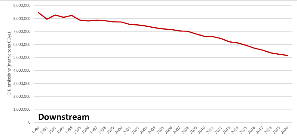
S-10
Figure S-6. Downstream CH
4
Emissions in New York State (AR5 GWP
20
)
The identified activity patterns correspond to national trends in CH
4
emissions. To validate this
emission inventory, comparisons were made with EPA’s nationwide inventory and with adjacent
state inventories. Comparison to the national inventory shows New York State CH
4
emissions to
be equivalent to 6.87% of the total national oil and natural gas inventory. Comparison with inventories
from adjacent states shows New York State oil and gas emissions to be approximately one-third of
emissions from the same source categories in Pennsylvania, which has much higher upstream
production and similar downstream consumption.

1
1 Introduction
In 2019, New York State passed the Climate Leadership and Community Protection Act (the Climate
Act). The Climate Act is among the most ambitious climate laws in the world and requires the State to
reduce economy-wide greenhouse gas (GHG) emissions 40% by 2030 and no less than 85% by 2050
from 1990 levels. The goal of this project is to support CH
4
emission reduction efforts in New York
State (NYS), and achievement of the Climate Act goals, by improving the State’s understanding of CH
4
emissions and CH
4
emissions-accounting methodologies for the oil and natural gas sector. The use of
improved accounting methodologies to develop an activity-driven, site-level, CH
4
emissions inventory
for upstream, midstream, and downstream sources is needed to inform mitigation strategies and measure
progress on fugitive CH
4
emission reductions from the oil and natural gas sector as the State moves
toward its ambitious climate goals. Consequently, the inventory developed under this project incorporates
findings from the most current empirical research and utilizes the most accurate, current, and inventory-
appropriate available data sources to develop an activity-driven, site-level, CH
4
emissions inventory.
The inventory developed under this project occurred in two phases. The project’s original phase sought
to update the New York State Greenhouse Gas (NYS GHG) Inventory 1990–2015 and implement the
following best practices to improve and develop an activity-driven, geospatially-resolved, CH
4
emissions
inventory for the oil and natural gas sector: (1) the use of appropriately scaled activity data, (2) inclusion
of state-of-the-science emission factors (EFs), (3) geospatial resolution of activities and emissions, and
(4) application and reporting of uncertainty factors, including high-emitting sources. To ensure project
rigor, a six-member Project Advisory Committee (PAC) comprised of experts with knowledge on air
pollutant emissions from the oil and natural gas sector was established to provide technical oversight and
peer review throughout the duration of the first phase of this project. The report for the initial phase was
published in 2019 and included data years 1990–2017. The current report represents the second phase of
this project, where updates were made to the new inventory to bring the data up to date through 2020 and
make improvements to emissions factors and additional sources.
Specific objectives of first phase of this project, completed in 2019, included (1) assessing the
State’s previous oil and natural gas sector CH
4
emissions inventory (NYSERDA and DEC 2018),
(2) performing a literature review of CH
4
emission-accounting methodologies and associated analyses
and studies, (3) developing an improved CH
4
emission-accounting methodology, and (4) implementing
the methodology to create an improved CH
4
emissions inventory for the oil and natural gas sector in
the State.
2
For Phase 2, further updates were made after the initial assessment and development of the NYS oil
and gas methane inventory. In addition to bringing the activity data up to date through 2020, additional
objectives during the second phase of the project included (1) assessing NYS’s 2017 oil and natural gas
sector CH
4
emissions inventory for areas of improvement, (2) performing a literature review of latest
data on fugitive oil and gas methane emissions in NYS, and (3) incorporating the latest data to create
an updated CH
4
emissions inventory for the oil and natural gas sector in NYS through 2020.

3
2 Characterization of New York State’s Oil and
Natural Gas Sector
The following section begins with a characterization of oil and gas wells, then moves into a discussion
of oil and gas production and concludes with an overview of associated oil and gas infrastructure.
2.1 Oil and Gas Wells in New York State
In 2020, New York State had 8,019 unplugged natural gas wells and 6,311 unplugged oil wells
(DEC 2021). In addition, the State had 9,637 plugged oil wells, 4,264 plugged gas wells (Figure 1),
825 unplugged storage wells, and 130 plugged storage wells. (Plugged wells are wells that are no
longer in use and the borehole has been plugged with cement or another impermeable substance to
isolate and prevent the underlying hydrocarbon formation from contaminating the environment.)
Figure 1. Number of Open Hole and Plugged Wells in New York State in 2020
Source: New York State Department of Environmental Conservation (DEC) downloadable well data.

4
Gas well development in New York State increased significantly in the 1970s, reaching a peak in
1982 when 611 wells were drilled and put into production, followed by a decline in activity until
the mid-2000s. There was a secondary spike in installations from 2006–2008 (Figure 2). After 2008,
natural gas well completions fell to fewer than 10 per year. High-volume hydraulic fracturing (HVHF),
or fracking, was banned in the State in 2014. Oil well completions also followed a cyclical pattern, with
increased activity from 1973–1985 and again from 2006–2014. Oil well completion activity follows oil
and natural gas price patterns, with higher activity during periods of high-fuel prices, and lower activity
during periods of low-fuel prices. The deregulation of oil and natural gas markets also played a role in
increasing production and consumption of natural gas while reducing prices.
Figure 2. Number of Oil and Natural Gas Wells Completed per Year in New York State
The age distribution of natural gas wells producing in New York State in 2020 (Figure 3) followed
a similar bimodal pattern to that seen in Figure 2. Well count data for 2020 show a primary peak of
wells aged around 12 and 13 years old, and a secondary peak of wells aged between 37 and 38 years
old. Comparing Figure 2 and Figure 3, age and completions follow a similar bimodal pattern, with peaks
in age corresponding to peaks in completions, indicating that older wells can remain in production for a
long time. Well age data showed that, although there were far more completions in the 1970s and 1980s,
14.7% of currently operational wells were completed in the last 15 years, with 88.4% of wells under
45 years old.

5
Figure 3. Age Distribution of Gas Wells Producing in 2020
2.2 New York State Oil and Natural Gas Production
Natural gas production far outweighs oil production in New York State as shown in Figure 4. Natural
gas production peaked at 55.34 billion cubic feet (Bcf) or 9.78 million barrels of oil equivalent (BOE) in
2006 (1 BOE = 5.65853 thousand cubic feet, Mcf), while oil production peaked at 386,192 barrels (bbl) in
2008. Natural gas production declined from 55.34 Bcf in 2006 to 10.70 Bcf, or 1.89 million BOE in 2020.
Oil production has also declined in the State from the 2008 peak to 146,861 bbl in 2020. Since there are
no in-state oil refineries, all the oil produced is refined out of State, primarily in Pennsylvania
(DEC 2006).
As shown in Figure 5, 157 out of 7,495 wells (2.09%) accounted for 50% of natural gas production in
New York State in 2020, 17.95% of the wells accounted for 75% of natural gas production, and almost
all (99%) of natural gas production came from 5,172 (69%) of wells. These data demonstrate that a
comparatively small number of wells produce the majority of natural gas, and that production is not
evenly distributed across those wells. Oil wells also showed a similarly skewed distribution, with
411 out of 4,963 (8.2 %) wells accounting for 50% of production, 864 (17.4%) wells accounting
for 75% of production, and 2,350 (47.4%) wells accounting for 99% of production in 2020.


7
Figure 5. Relationship between Percent of Total Cumulative Oil and Natural Gas Production in
2020 and the Number of Wells in New York State
As shown in Figure 6, oil and natural gas production occur largely in Western New York, west of the
line delineating the eastern boundary of Broome, Chenango, Madison, Oneida, and Lewis counties.
Oil production is concentrated in the far west of New York State, in Allegany, Cattaraugus, Chautauqua,
Erie, and Steuben counties.

8
Figure 6. Oil and Natural Gas Well Locations and Production in New York State in 2020
(Oil): *There are no oil producing wells located outside of western New York.
(Natural
Gas)

9
2.3 New York State Oil and Natural Gas Infrastructure
As shown in Figure 7, oil and natural gas activities are concentrated in the western portion of the State.
Western NY has the greatest density of wells and underground natural gas storage facilities. Storage
fields are located in former solution salt caverns and depleted reservoirs. The Energy Information
Administration (EIA) data lists no natural gas processing plants in New York State, with the closest
processing plants located in northwestern Pennsylvania. The greatest density of interstate and intrastate
natural gas transmission pipelines, as identified by EIA, is in Western New York near the production and
storage wells for removal and delivery. Transmission pipelines are well-connected to Pennsylvania and
have linkages to Canada in the west and north. Two main pipeline trunks extend east-west across the
State, with one along the southern Pennsylvania border, connecting to pipelines in the New York City
Metropolitan Area and the other connecting farther north to pipelines in the Albany and Buffalo regions.
Figure 7. Locations of Oil and Natural Gas Wells, Natural Gas Processing Plants, Natural
Gas Pipelines, Natural Gas Underground Storage, and Shale Plays in New York State and
Surrounding States

10
New York State has 17 natural gas utility service territories (Figure 8). These service territories cover
around 94% of the households identified by the United States (U.S.) Census Bureau. According to the
Census, 54% of households inside natural gas utility service areas use natural gas as their primary home
heating source. In addition, EIA data
2
show 422,542 commercial and industrial end users of natural gas
in the State. Based on census data, which show 537,369 registered businesses in 2020 with 96.9% of
businesses within natural gas utility service areas, 81.1% of businesses inside natural gas utility
service areas use natural gas.
Figure 8. New York State Gas Utility Service Territories

11
3
Methane
Emissions
Inventory
Development
3.1
Methane
Emissions
Literature
Review
3.1.1 Overview
The following section provides the results of a literature review, primarily conducted during Phase 1
of the project, aimed at uncovering best practices for CH
4
inventory development and inputs to inform
improvements in the State’s inventory models in the future.
As part of Phase 1, a literature review was conducted that included peer-reviewed articles, reports,
and tools describing state-of-the-art CH
4
inventory development in the United States and internationally,
with a focus on emissions in the oil and natural gas sector. While over 100 documents on oil and natural
gas emissions were carefully reviewed, specific attention was paid to three sources of information:
(1) EPA’s GHGRP (Greenhouse Gas Reporting Program) Subpart W, (2) EPA’s FLIGHT (Facility
Level Information on GreenHouse gases Tool), and (3) the Environmental Defense Fund’s (EDF)
16 Study Series. The European Union’s (EU) most recent inventory report (European Environment
Agency 2018) was also reviewed to explore differences between international and U.S.-centric
inventory methodologies.
The literature review highlights the
rapid advancement of state-of-the-art CH
4
inventory development.
In just the last decade, new data now allow for more geographic-specific inventory development and
greater certainty of emissions, ranging from routine leaks to episodic releases. The literature has also
advanced on identifying the role of high-emitting sources, which have previously been ignored in
conventional CH
4
inventories, but which can play an important part in a region’s overall emission
levels. The literature review was used to inform the first iteration of the New York State Oil and
Gas Methane Emissions Inventory (NYSERDA 2019).
Section 3.1.2 presents key terminology so that readers may better understand subsequent sections.
Section 3.1.3 reviews existing methane inventory approaches for oil and natural gas systems. Section
3.1.4 discusses key findings on emission factors, spatial variability, and high-emitting sources. Section
3.2 provides a review of the methods and data used to develop this inventory including a summary of best
practices, assessment of emissions factor confidence, an activity data summary, and a review of emission
factor development for the upstream stages, midstream stages, and downstream stages.
12
3.1.2
Key
Terminology
3.1.2.1 Oil and Natural Gas Supply Chain
The U.S. oil and natural gas supply chain can be broken into nine main segments. For oil development,
CH
4
emissions occur across the following four stages: (1) exploration, (2) production, (3) gathering and
boosting, and (4) transmission. For natural gas development, CH
4
emissions occur across the following
nine stages: (1) exploration, (2) production, (3) gathering and boosting, (4) processing, (5) transmission,
(6) underground storage, (7) LNG import and export terminals, (8) LNG storage, and (9) distribution,
as shown in Figure 9 (Howarth 2014; Harrison et al. 1997a). These stages are divided into three major
groups: (1) upstream, (2) midstream, and (3) downstream stages.
3.1.2.2 Upstream Stages
• Exploration includes well drilling, testing, and completions. The predominant sources of
emissions from exploration are well completions and testing.
• Production involves taking crude oil or raw natural gas from underground formations, whether
using conventional drilling or unconventional drilling techniques. Sources of emissions during
the oil production stage typically include leaks, pneumatic devises, storage tanks, and flaring
of associated gases. Sources of emissions during the natural gas production stage depend
on the technologies employed for gas extraction, but typically include leaks, pneumatic
controllers, unloading liquids from wells, storage tanks, dehydrators, and compressors.
Many wells co-produce oil and natural gas; therefore, the distinction between oil
production and gas production is not always clear.
• Gathering and boosting stations receive natural gas from production sites/wells and via
gathering pipelines, and then transfer the gas to transmission pipelines and/or processing
facilities and distribution systems. Compression, dehydration, and sweetening (removal
of foul-smelling sulfur containing compounds) occur in this segment. Sources of emissions
in this segment include gathering stations, pneumatic controllers, natural gas engines,
gathering pipelines, liquids unloading, and flaring.
3.1.2.3 Midstream Stages
• Natural gas processing includes the process of removing impurities and other hydrocarbons,
including liquids, from raw natural gas, resulting in pipeline grade natural gas. Emissions from
the processing stage originate from reciprocating and centrifugal compressors, blowdowns,
venting, and leaks.
13
• The transmission and compression stage is the transfer of natural gas from gathering lines and
processing plants to the city gate or to high-volume industrial users through main transmission
lines. Compressor stations located along the pipelines maintain high pressure and move the gas
throughout the system. Sources of emissions in this segment include compressor stations,
venting from pneumatic controllers, uncombusted engine exhaust, unburned and
pipeline venting.
• Underground storage involves injecting natural gas into underground formations during
periods of low demand; and the natural gas is withdrawn, processed, and redistributed during
periods of high demand. Compressors and dehydrators are the primary emission sources from
the storage segment.
• LNG import/export terminal activities involve the receipt and delivery of LNG for storage
and ultimately delivery.
• LNG storage involves the storage of LNG while it awaits final distribution.
3.1.2.4 Downstream Stage
• The distribution stage represents the delivery of natural gas to end users through distribution
mains and service pipelines. Distribution pipelines receive high-pressure gas from the
transmission pipelines at city gate stations, where the pressure is reduced, and the gas is
distributed through predominantly underground main and service pipelines to the customer’s
meter, where the downstream stage ends. Primary sources of emissions from the distribution
segment are leaks from pipes and metering and regulating (M&R) stations. Fugitive emissions
after the customer meter are not considered here since those emissions should be accounted
for in the residential or commercial sector inventory.
• Beyond-the-meter end use sources are those downstream of meters, and account for end-uses
such as natural gas appliances and commercial and residential buildings. Discrepancies between
top-down and bottom-up methodologies (see section 3.1.2.6) suggest that beyond-the-meter
sources are a significant contribution to methane emissions.

14
Figure 9. Oil and Natural Gas System Depicting the Upstream, Midstream, and Downstream
Grouping of Stages
The fraction of emissions is based on the 2014 EPA U.S. GHG Inventory.
Source: McCabe et al. 2015.
15
3.1.2.5 Emission Source Categories
Emissions from oil and natural gas production systems fall into three main categories: fugitive
emissions, vented emissions, and combustion emissions (Kirchgessner 1997). Definitions of
these categories are as follows:
• Fugitive emissions represent unintended emissions from equipment leaks (such as those from
compressor stations, meters, pressure regulating stations, malfunctioning pneumatic controllers,
and various parts of the production process) and pipeline leaks due to deteriorating pipelines
or poor pipeline connectors.
• Vented emissions represent purposeful releases (i.e., by design) of CH
4
(e.g., through
pneumatics, dehydrator vents, regular maintenance, and chemical injection pumps).
• Combustion emissions represent unburned CH
4
emitted during any fossil fuel combustion
component of the production process (e.g., compressor exhaust emissions or flares).
These different types of emissions are discussed in the context of inventory development in the
following sections.
3.1.2.6 Bottom-Up versus Top-Down Methodologies
CH
4
emissions from the oil and natural gas sector are typically quantified using either top-down (TD)
or bottom-up (BU) methodologies. Definitions of these methodologies are as follows:
• TD studies calculate CH
4
emission levels using observational techniques, including
airborne measurements, satellites, mobile measurement devices, and stationary sensors.
These approaches estimate aggregate CH
4
emissions from all sources in a given region, and
then attempt to apportion those emissions to different source categories. Allen (2014) notes
that the challenges of estimating emissions using TD methods include separating anthropogenic
emissions from natural emissions, and identifying legacy emission sources such as abandoned
wells and nonoperational infrastructure. TD estimates are typically generated at the area-level.
• BU studies generate emission estimates by applying EFs to different activities in the oil and
natural gas sector. The generation of EFs can be challenging and usually involve laboratory
or in situ measurements of emissions that are then extrapolated and applied broadly to develop
overall emission inventories. As Allen (2014, 2016) notes, one of the primary challenges with
BU studies is obtaining a representative sample of a large, geographically dispersed, and diverse
population of equipment and activities. Other uncertainties are due to inaccurate activity data,
malfunctioning equipment, or poorly operated equipment (Allen 2016). Furthermore, emissions
from various sources are not normally distributed, and so the use of an “average” EF may lead
to both overestimation and underestimation (Littlefield et al. 2017). BU inventories are typically
estimated at the component or site level. BU estimates are particularly challenging when
estimating emissions from high-emitting sources, as an accurate estimate requires either
prior understanding of which sources are likely to be high-emitting sources; or obtaining a
statistically representative sample, which is itself not easily determined without a large
16
sample size. Lastly, because BU methods calculated at the component level only capture
source emissions for known and well-defined sources, they typically underestimate actual
emissions, which include emissions from unknown or ill-defined sources (Heath et al. 2015;
Adam R Brandt, Heath, and Cooley 2016; A R Brandt et al. 2014; Miller et al. 2013;
Alvarez et al. 2018).
• Site-level estimates use a similar methodology to TD estimates, often estimating emissions
from atmospheric concentrations, but then apply those estimates in a BU approach. Site-level
estimates are generated for each site (e.g., well head, compressor station) and are at a smaller
geographic scale than TD estimates—and at a greater scale than component-level BU estimates.
In both BU and TD approaches, uncertainty exists and the literature suggests that CH
4
inventories at
the national level are likely under representing actual emissions by 50% or more (Miller et al. 2013;
A R Brandt et al. 2014). At a regional level, Miller et al. (2013) suggest that fossil fuel extraction and
processing emissions could be three to seven times higher than reported. Zavala-Araiza et al. (2015a)
also show that CH
4
emissions from oil and gas production are almost twice as large as reported by the
EPA and represent approximately 1.5% of natural gas production. This 1.5% may also be on the low
range; other authors have observed regional losses of 2–12% or more in the Natural Gas sector, implying
CH
4
emissions nationally could be three times higher than the EPA reports (Pétron et al. 2012; A.
Karion et al. 2013; Caulton et al. 2014). The ceiling for fugitive emissions can be considered as the
delta between aggregated meter readings in the distribution segment and the input of gas into the
system from production and gathering.
3.1.3
Review of Existing Methane Inventory Approaches for Oil and
Natural
Gas Systems
3.1.3.1 EPA’s Greenhouse Gas Reporting Program Subpart W
EPA’s GHGRP [codified at 40 Code of Federal Regulation (CFR) Part 98] requires large emitters
of GHGs to report their emissions through a centralized database accessible by the public (EPA n.d.).
Data collection began in 2011 and covers sources emitting over 25,000 MT of CO
2
e per year, using
the GWP
100
from AR4 (IPCC 2006) for converting CH
4
and other GHGs to CO
2
e. These facilities
self-identify and report annually. The owners and operators of these facilities are tasked with
calculating CO
2
e emissions, filing their results with the EPA, and maintaining records.
17
Subpart W of the GHGRP is focused specifically on facilities operating in oil or gas sectors (EPA 2018a).
This includes emission sources in the following segments of the oil and natural gas system. Subpart W
facility definitions differ across segments and are defined in parentheses.
• Onshore Oil and Natural Gas Production (Company or Basin)
• Offshore Oil and Natural Gas Production (Company or Basin)
• Natural Gas Gathering and Boosting (Company or Basin)
• Natural Gas Processing (Site)
• Natural Gas Transmission Compression (Site)
• Natural Gas Transmission Pipeline (Site)
• Underground Natural Gas Storage (Site)
• LNG Import/Export (Site)
• LNG Storage (Site)
• Natural Gas Distribution (Company or State)
In 2016, 2,248 Subpart W facilities reported emissions totaling 282.9 MMTCO
2
e, of which
186.7 MMTCO
2
e was CO
2
, 96.0 MMTCO
2
e was CH
4
, and 0.2 MMTCO
2
e nitrous oxide (N
2
O).
Note that although the GHGRP data and the U.S. national GHG Inventory are not directly comparable,
total emissions in the U.S. for all sectors in 2016 was 6,511 MMTCO
2
e (EPA 2018a), so the Subpart W
emitters contributed about 4.3% of total emissions nationally.
GHGRP facilities are required to report emissions greater than 25,000 MTCO
2
e for specific source
categories. Facilities report emissions data to the EPA through an electronic submission. A review
of the spreadsheet tool used by the EPA for this purpose, herein called the “Subpart W Tool,” was
conducted. The Subpart W Tool is a BU approach that captures emissions of different components
of the oil and natural gas system. The Subpart W forms are embedded in a Microsoft Excel spreadsheet
and require facilities to provide input on equipment at an operational level. For example, Subpart W
forms ask for input on the quantity of oil and natural gas produced, the quantity of oil and natural gas
stored, the number and type of pneumatic devices and pumps, the number and types of dehydrators,
the amount of well venting for liquids unloading, blowdown vent stacks, well completions, atmospheric
storage units, flare stacks, and estimates of non-planned emission leaks.
The value of the Subpart W form for inventory development is its library of EFs, which provide
specific values for a host of equipment and operations. For example, onshore production facilities
that use natural gas pneumatic devices will find EFs (standard cubic feet/hour/device) for high-bleed
pneumatic devices, intermittent-bleed pneumatic devices, and low-bleed pneumatic devices of 37.9,
13.5, and 1.39, respectively. This level of detail is useful for others constructing BU emission inventories.
18
3.1.3.2 EPA’s Facility-Level Information on Greenhouse Gas Tool
EPA’s FLIGHT provides access to GHG data reported to the EPA through the previously mentioned
Subpart W reporting system and other GHGRP subparts. Aside from providing data access in geospatial,
graphical, and tabular formats, FLIGHT does not provide any additional advancements with respect to
inventory methodology.
3
Data included in FLIGHT are submitted to the EPA periodically under the GHGRP (typically in
March following the reporting year), as reported by over 8,000 facilities, including Subpart W and
non-Subpart W facilities. These data are submitted by large emitters (> 25,000 MMTCO
2
e.yr
-1
) and
cover an estimated 85–90% of total GHG emissions in many sectors in the U.S., including power
plants and landfills, but less than 50% of the oil and natural gas sector. GHGRP data are available
at the national, state, local, sector, and facility levels (EPA 2018c).
Emission sources available in FLIGHT relevant to CH
4
inventory accounting include point sources,
onshore oil and gas production, onshore oil and gas gathering and boosting, local distribution, and
onshore gas transmission pipelines. Sectors available in FLIGHT are power plants, petroleum and
natural gas systems, refineries, chemicals, other, minerals, waste, metals, and pulp and paper.
EPA’s Envirofacts, which draws on data from EPA’s GHGRP and provides an alternate path to
accessing FLIGHT data, shows that CH
4
emissions from all sources in New York State in 2016 totaled
3,082,129 MTCO
2
e (using IPCC AR4 GWP
100
values), of which 1,334,090 MTCO
2
e of CH
4
were
emitted from the oil and natural gas sector, and 1,716,960 MTCO
2
e were emitted from waste facilities,
primarily landfills (the agriculture sector was not included). Together, these two sectors account for
98.98% of non-agriculture based CH
4
emissions reported in the State (43.28% and 55.70%, respectively).
3.1.3.3 EPA’s Greenhouse Gas Emissions Inventory
EPA’s Inventory of U.S. Greenhouse Gas Emissions and Sinks: 1990–2016 provides an overview
of U.S. GHG emissions, including CH
4
emissions from oil and natural gas systems (EPA 2018a).
The approach for calculating emissions for natural gas systems generally involves the application
of EFs to activity data. For most sources, the approach uses technology specific EFs or EFs that vary
over time and consider changes to technologies and practices, which are used to calculate net emissions
directly. For others, the approach uses what are considered “potential methane factors” and reduction
data to calculate net emissions.
19
Key references for EFs for CH
4
emissions from the U.S. oil and natural gas sector include a 1996
study published by the Gas Research Institute (GRI) and the EPA (EPA/GRI 1996). The EPA/GRI
study developed over 80 CH
4
EFs to characterize emissions from the various components within the
operating stages of the U.S. natural gas system. The EPA/GRI study was based on a combination of
process engineering studies, a collection of activity data, and measurements at representative gas
facilities conducted in the early 1990s.
In the production segment, EPA’s GHGRP data (EPA 2017) were used to develop EFs used for all years
for well testing, gas well completions and workovers with and without hydraulic fracturing, pneumatic
controllers and chemical injection pumps, condensate tanks, liquids unloading, and miscellaneous flaring.
In the processing segment, for recent years of the times series, GHGRP data were used to develop EFs
for fugitives, compressors, flares, dehydrators, and blowdowns/venting. In the transmission and storage
segment, for recent years of the times series, GHGRP data were used to develop factors for pneumatic
controllers. Other data sources used for CH
4
EFs include Marchese et al. (2015) for gathering stations,
Zimmerle et al. (2015) for transmission and storage station fugitives and compressors, and Lamb et al.
(2015) for recent years for distribution pipelines and meter/regulator stations. When changes are made to
the EPA GHG Inventory methodology, the EPA adjusts inventories from prior years to be consistent with
the updated methodology.
3.1.3.4 Environmental Defense Fund’s 16 Study Series
The Environmental Defense Fund (EDF) has been a leader in undertaking investigations into CH
4
emissions in the oil and natural gas sector (EDF 2018). Through this work, EDF has drawn attention
to factors such as leakage rates from aging equipment or poor operations, episodic emissions due to
equipment failures, and high-emitting sources. EDF has also been a leading proponent of considering
alternative GWP values when conducting GHG emission analyses, noting that the selection of an
appropriate GWP depends on the types of environmental problems one is trying to address, and that
the relatively arbitrary selection of a GWP
100
may be inferior to a GWP
20
, especially when considering
the importance of short-term climate impacts (Alvarez et al. 2018).
20
With respect to supply chain analysis, EDF has been working since 2012 on a number of projects
aimed at providing a peer reviewed, scientific basis for assessing CH
4
emissions in natural gas supply
systems. The research program is divided into 16 different areas, hence the “16 Study Series” moniker.
This section of the report summarizes the results to date from EDF’s work. A summary of each of the
16 studies is shown in Table 1. These studies are useful in helping identify important issues, EFs, and
areas of uncertainty for future inventory work for New York State.

21
Table 1. List of Studies Included in Environmental Defense Fund’s 16 Study Series (2018)
Study
Area/Title
Overview
of
Results
References
Production Studies
Natural Gas
Production
Site
Emissions
Conducted measurements of
CH
4
emissions at natural gas production sites (convention al and
hydraulically fractured wells). Found that
CH
4
emissions over an entire completion flowback event
ranged from less than 0.1 megagram (Mg) to more than 17 Mg, with a
mean of 1.7 Mg [0.67-3.3 Mg
with a 95% Confidence Interval (CI)]. Results show that wells with
CH
4
capture and/or control devices
captured 99% of the potential emissions, and that 3% of the wells account for 50% of estimated
emissions during unloading.
Allen et al. 2013
Identified that due to a possible malfunction, the Bacharach Hi Flow® Sampler (BHFS) may
underestimate
C
H
4
emissions by as much as 40-80%. The authors constrained the potential
underestimate and, given differences in flow rates and
CH
4
content across different sites, they
estimate
that emissions from the Natural Gas Production sector may be 7
–14% greater than initially thought,
with total supply chain emissions being 2
–5% greater.
Alvarez et al. 2016
Production Site
Emissions
Reviewed emissions from 377 gas actuated (pneumatic) controllers at natural gas production sites and
a small number of oil
production sites. Found that 19% of devices accounted for 95% of entire gas
emission rates, with significant geogra
phic variation. Gulf Coast
CH
4
emission rates were the highest
[10.61 standard cubic foot (scf)/hr] followed by mid
-continent (4.87 scf/hr), Appalachian (1.65 scf/hr),
and Rocky Mountain (0.67 scf/hr) emission rates. The highest
-emitting devices were shown to be
behaving in a manner inconsistent with their design specifications.
Allen, Pacsi, et al. 2015
Additional Data
Investigated
CH
4
emissions from wells during liquid unloading events. Liquid unloadings to clear wells
of accumulated liquids to increase production may be necessary when a gas well also produces water.
Wells with plunger lifts are triggered to unload far
more frequently than wells without plunger lifts
(thousands of times per year v
ersus less than 10 times per year). Though wells without plunger lifts
emit more
CH
4
per unloading event (0.4–0.7 Mg) than wells with plunger lifts (0.02–0.2 Mg), the
frequency
of unloading events means that wells with plunger lifts account for the majority of CH
4
emissions from liquid unloading. Twenty percent of wells sampled with plunger lifts account for 83%
of emissions. With plunger lifts, 20% of wells account for 65
–72% of annual emissions (manual and
automatically triggered, respectively).
Allen, Sullivan, et al. 2015
Production
Studies
Production Data
Analysis
Developed a multivariate linear regression to test the relationship of well ag e, gas production, and oil
or condensate production to CH
4
emissions:
log
(
CH
4
)
=
1
log
(
gas
)
+
2
log(oil)
+
3
age
Age was not significantly correlated with C
H
4
production while gas production was significantly
positively correlated [
\beta_1 = 0.25 (p < 0.001)], and oil production was significantly negatively
correlated [
\beta_2 = -0.08 (p = 0.01)]. Emissions showed significant geographical variation by basin.
Brantley et al. 2014

22
Table 1 Continued
Study Area/Title
Overview of Results
References
Midstream Studies
Gathering and
Processing Study
Measurements at 114 gathering facilities and 16 processing plants showed
CH
4
emissions ranging
from 0.7 to 700 kg/
hr
-1
.
Thirty percent of gathering facilities contributed 80% of total emissions, and
normalized emissions are negatively correlated with facil
ity throughput, though higher throughput is
positively correlated with
CH
4
emissions. Venting from liquids storage tanks occurred at ~ 20% of
facilities, which showed four times the emission rates of similar facilities without substantial venting.
Mitchell et al. 2015
Marchese et al. (2015) used the results from Mitchell et al. (2015), combined with state and national
facility databases, to develop a Monte Carlo simulation to estimate
CH
4
emissions from U.S. natural
gas gathering and processing operations. Total annual
CH
4
emissions of 2,421 (+245/-237)
gigagrams (Gg) were estimated for all U.S. gathering and processing operations, representing a
CH
4
loss rate of 0.47% (± 0.05%) when normalized by annual
CH
4
production. Ninety percent of those
emissions are attributed to
normal operation of gathering facilities. CH
4
from gathering facilities are
substantially higher than prior EPA estimates and are equivalent to ~ 30% of total net
CH
4
emissions
from natural gas systems in the current GHG Inventory. Results showed substant
ial variation in
losses by state, with the highest loss rates in Oklahoma (0.94%) and the lowest in Pennsylvania
(0.19%). A facility
-level EF for gathering stations (42.6 kg/hr/facility) and estimated number of U.S.
gathering stations (4,459 facilities) fr
om this study were incorporated into the EPA GHG Inventory in
April 2016.
Marchese et al. 2015
Transmission and
Storage Study
Data from 45 compressor stations in the Transmission and Storage sector showed highly skewed
site
-level CH
4
emissions, with 10% of sites contributing 50% of CH4 emissions. The range in
emissions observed is 1.7 ± 0.2 standard cubic foot per minute (SCFM) to 880 ± 120 SCFM, with the
highest emissions generated by two high
-emitting sites. Sites with reciprocating
compressors showed
typically greater emissions than sites with only centrifugal compressors.
Subramanian et al. 2015
Evaluated CH
4
emissions from the Transmission and Storage sector. The largest emission sources
were high
-emitting sources, which showed site-level emission rates that were much higher than their
aggregate component
-level emission rates. In this instance, these high-emitting sources showed
anomalous operations, such as leaking isolation valves, etc. Overall, on a per
-
station level, emissions
from underground storage compressor stations were 847 Mg
·station
-1
·yr
-1
(+53%/-35%) and
transmission stations were 670 Mg
·station
-1
·yr
-1
(+53%/-34%). Sup er-emitters contribute 39% of
transmission fugitives and 36% of storage station fugitives, highlighting the importance of observing
high
-emitting sources, and modeled sup er-emitters are better modeled as frequency of occurrence
rather than based on equipment counts.
Zimmerle et al. 2015

23
Table 1 continued
Study Area/Title
Overview of Results
References
Local Distribution Studies
Multi
-City Local
Distribution Study
Direct measurements of 230 underground pipeline leaks and 229 metering/re
gulating facilities
showed that emissions from leaks are generally lower (~ 2 times) than those described earlier in
1992, with a similar pattern in M&R facilities.
Annual CH
4
emissions were calculated by multiplying
the number of leaks in each category by the appropriate EF. Leaks in cast
-iron and unprotected steel
pipe account for 70% of eastern emissions and almost half of total U.S. emissions.
Lamb et al. 2015
Boston
Study
Atmospheric study that showed overall emissions of 18.5 ± 3.7 g
CH
4
m-2 r
-1
. Natural gas
emissions rate is 2.7 ± 0.6% of consumed natural gas in Boston, which is ~ 2
-3 times greater
than prior estimates.
McKain et al. 2015
Indianapolis
Study
Atmospheric study with observed emissions from distribution, metering, regulating, and pipeline leaks
showed 48% of emissions were from biogenic sources, and 52% of emissions from natural gas
usage. Mean observed leak rates from pipelines were 2.4 g
min
-1
(range of 0.013 g min
-1
to
22.3 g
min
-1
).
Lamb et al. 2015
Methane Mapping
Mobile analysis
using vehicle-based sensors showed cities with a greater prevalence of corrosion-
prone distribution lines (~ 25 times larger). Eliminating 8% of leaks would reduce gas
pipeline
emissions by up to 30%, and the largest 20% of leaks account for half of all em
issions.
Von Fischer et al. 2017
Basin-Specific Studies
Denver
- Julesburg
(D
-J) Basin
Using ground
-based and airborne measurements of the D-J Basin, study showed that non-
oil and gas
sources contribute around 7.1 ± 1.7 MT CH
4
h
-1
(May 29) and 6.3 ± 1.0 MT CH
4
h
-1
(May 31) or 24-
27.5% of total measurement based CH
4
emissions. Non-oil and gas sources include animals, animal
waste, landfills, municipal wastewater plants, and industrial wastewater plants.
Pétron et al. 2014
Barnett
Study
Extensive set of work that used air and ground measurements to develop CH
4
emission estimates
for oil and gas wells in the Barnett Shale in Texas. Results indicated emissions were 50
–90% higher
than would have been predicted using EPA’s GHG
Inventory model.
Yacovitch et al.
2015 Rella et al. 2015
Nathan et al. 2015 Harriss et al. 2015
Lyon et al. 2015
Zavala-Araiza, Lyon, Alvarez,
Palacios, et al. 2015
Smith et al. 2015
Johnson, Covington, and Clark 2015
Lavoie et al. 2015
Townsend-Small et al. 2015
Zavala-Araiza, Lyon, Alvarez, Davis,
et al. 2015a
Zavala-Araiza et al. 2017

24
Table 1 continued
Study Area/Title
Overview of Results
References
Basin-Specific Studies
Flyover
Study:
Barnett Shale
Involved aircraft
measurements of hydrocarbons over the Barnett Shale to quantify regional CH
4
emissions.
Karion et al. 2015
Other
Studies
Pump
-to- Wheels
Assessed CH
4
emissions from medium- and heavy-duty vehicles operating on natural gas. The
research also included assessments of CH
4
emissions through liquefied and compressed natural gas
refueling. CH
4
emissions from vehicle tailpipes (30%) and crank cases (39%) were the dominate
emission sources, while refueling emissions were relatively low (12% of transport segment
emissions).
Clark et al. 2017
Pilot
Projects
EDF funded a number of
pilot projects that helped informed the research threads included in this
table Although no references are given for these pilot projects
per se, the results of the projects are
embedded in the work referenced throughout this table.
NA
Filling Gaps,
Incl
uding
Super
-Emitters
Identified high
-
emitting sources from a set of 8,000 well pads using aerial flyovers and to estimate the
contribution of CH
4
emissions by abandoned wells using a set of 138 abandoned oil and gas wells in
4 basins. These high
-emitting sources represent sources that disproportionately contribute to
emission inventories. Lyon et al. (2016) concluded that high
-emitting sources are “widespread and
unpredictable” but easily identifiable with appropriate monitoring systems. Townsend
-Small et al.
(2016) estimated that abandoned wells contribute less than 1% to regional CH
4
emissions in the
study areas.
Lyon et al. 2016
Townsend-Small et al. 2016
Project
Synthesis
A synthesis of the current state of knowledge around CH
4
emissions from natural gas production, with
input from numerous stakeholders, was conducted; the conclusions indicate that actual emissions of
CH
4
may be ~ 60% higher than currently reported in official U.S. inventories, and that 2.3% of the
CH
4
in natural gas is emitted between extraction and delivery.
Littlefield et al. 2017 Alvarez et al.
2018
25
3.1.3.5 European Union’s Greenhouse Gas Inventory
A review was performed on the inventory approaches implemented by the EU, as discussed in the Annual
European Union Greenhouse Gas Inventory 1990–2016 and Inventory Report 2018 (EU Inventory)
through the European Environment Agency 2018.
4
The EU Inventory applies methodologies outlined
by the IPCC in 2006 and uses GWP information contained in AR4.
5
The EU Inventory is essentially an
amalgamation of inventories for each of the 28 EU member nations plus Iceland. Each nation is allowed
flexibility in its methodological approach, as long as it follows IPCC guidance. That guidance outlines
three tiers of methodologies, representing increasing complexity and certainty. For example, Tier 1
methods are TD and apply average EU EFs (e.g., gCO
2
e/MBTU natural gas) to national activity data
(e.g., MBTU of natural gas consumed). Upon review of the EU Inventory and country specific EFs, the
data show that using EFs from the U.S. is more applicable to the New York State context. Tier 2 applies
more nationally focused EFs and activity data, but still represents a TD approach, and Tier 3 represents
significant BU analysis, where production and consumption systems are well-defined at the equipment
level, and emissions are calculated through equations that depict activity at the micro-level, similar to
the Subpart W analysis previously mentioned (IPCC 2006, Vol 2, Ch. 4). Tier 1, 2, and 3 approaches
are described in more detail in the following passages.
The EU Inventory estimates gaseous emissions in four source categories in IPCC’s Common Reporting
Framework Source Category 1.B related to fossil fuel extraction, handling, and consumption. These
are Coal Mining and Handling (1.B.1.a), Oil (1.B.2.a), Natural Gas (1.B.2.b), and Venting and Flaring
(1.B.2.c). Source category 1.B.2 (a and b) is the EU equivalent to the U.S. Oil and Natural Gas
Production and Infrastructure sector. The EU GHG Inventory reports that 70.6% of emissions from
Source Category 1.B are from fugitive CH
4
emissions, while 29.3% are fugitive CO2 emissions.
The Tier 1 methodology involves the application of appropriate default EFs to a representative activity
parameter, often natural gas throughput, to each segment or subcategory of the country’s oil and natural
gas industry. The set of equations applied here is a simple scaling of activity estimates by an EF, summed
across industry segments. A major flaw of this approach is that emission intensities are fixed relative to
activity levels and do not reflect changes in emissions that may result from efficiency improvements and
infrastructure upgrades over time.
26
The Tier 2 methodology applies the same general approach as Tier 1 but applies country-specific EFs
that were developed from studies and measurement programs specific to the country’s infrastructure.
Best practices suggest that Tier 2 EFs be updated periodically. Where reliable venting and flaring data
are available, a country may use an alternative Tier 2 approach, which also factors in emissions due to
venting and flaring through a set of defined equations (IPCC 2006). This alternative approach may be
used to estimate emissions due to venting and flaring from oil production.
The Tier 3 methodology applies a rigorous BU assessment of primary emission sources at the facility
level. This approach requires a high level of detail on facilities, wells, flare and vent processes,
production, reported and measured releases (planned and unplanned), and country-specific EFs.
These inventories require a significant level of effort, and it is common among EU countries to
periodically produce Tier 3 inventories, and then use these detailed studies to back-calculate the
EFs, which can then be used in interim years’ Tier 2 studies.
Data from the EU Inventory indicate that fugitive CH
4
emissions from natural gas (Source
Category 1.B.2.b) account for 0.6% of total EU – 28 + ISL (28 EU countries, plus Iceland)
GHG emissions, and account for 30% of all fugitive emissions. Fugitive sources include
exploration, production, processing, transmission, and storage and distribution of natural gas.
Fugitive CH
4
emissions from oil (Source Category 1.B.2.a) account for 0.1% of total EU – 28 + ISL
GHG emissions and 4% of all fugitive emissions. Fugitive emissions from oil are associated with
exploration, production, transmission, upgrading and refining of crude oil, and distribution of crude
oil products.
Data for Source Category 1.B.2.b were calculated at the EU country level using a range of
methodologies, from Tier 1 to Tier 3 methods, as prescribed by the IPCC in 2006 (IPCC 2006). Data
for Source Category 1.B.2.a were calculated at the EU country level using Tier 1 and Tier 2 methods.
The decision trees provided by the IPCC for determining which methodology to apply for each source
category are shown in Figure 10 and Figure 11. The decision trees are provided here because they may
offer useful guidance as the State considers different approaches to inventory development.

27
Figure 10. Decision Tree for Determining Natural Gas System Fugitive CH
4
Emissions
Estimation Methodology
Source: Figure 4.2.1 from IPCC (2006).

28
Figure 11. Decision Tree for Determining Oil System Fugitive CH
4
Emissions Estimation
Methodology
Source: Figure 4.2.2 from IPCC (2006).
29
3.1.4
Emission
Factors, Spatial Variability, and High-Emitting Sources
3.1.4.1 Emission Factors
One of the most important inputs for CH
4
inventories is the identification of appropriate EFs for BU
analyses. These EFs are applied to different activities to calculate emission inventories at either (1) a
national, regional, or state basis, or Tier 2 analyses, or (2) a process and system level, or Tier 3 analyses.
In its simplest form, an example of a Tier 2 type of calculation is shown in the following equation,
where E
s,i
is the emissions of type i for period s, NG
s
is the natural gas consumption (or throughput)
in period s in SCF, and EF
i
is the EF for emissions of type i in mass⋅SCF
-1
.
Equation
1
,
=
Tier 2 approaches allow reporting facilities or organizations to easily prepare inventories in cases where
limited data exist. EFs for Tier 2 analyses are generally estimated by sampling or testing a set of devices,
processes, and facilities; generating EFs at a component level; and then synthesizing those EFs so that
they can be applied more widely. Although simple to use, the drawback is that EFs for Tier 2 analyses
are averages based on sample testing and may not reflect the actual emissions of the particular facility
or region under study.
Tier 3 analyses are more site-specific and estimate emissions at a facility level by incorporating data at
an operational level. An example of a type of Tier 3 analysis is shown in the following equation, which
is used by facilities to estimate emissions from three types of pneumatic devices using EPA’s Subpart W
inventory tool mentioned previously.
Equation
2
,
=
where:
• E
s,i
is emissions of type i for year period s
• N
t
is the number of devices of type t
• EF
t
is the EF for device of type t measured in SCF⋅hr
-1
⋅device
-1
• GHG
i
is the concentration of GHG of type i in natural gas as a percent
• T
t
is the average number of hours during the period the devices were operating

30
Although Tier 3 analyses use more specific facility and operational data (i.e., activity data) when
calculating emissions, the EFs used may not reflect actual EFs for the facility. Thus, in both Tier 2
and Tier 3 analyses, the selection of an appropriate EF is critically important, as emissions are
directly and proportionally related to these values.
What has emerged in the literature is an evolution of EFs over time, informed by ongoing
research, testing, and demonstration projects. As an example of that variability, data from Howarth
(2014) that summarize CH
4
emissions as a percentage of natural gas throughput by process stage
(upstream/downstream) and type of natural gas extraction (conventional/unconventional) are
reproduced in Table 2.
Table 2. Information on EFs (as a percentage loss) for Upstream, Downstream, and Total
Based on Data in Howarth (2014)
Source
Upstream
Conventional (%)
Upstream
Unconventional (%)
Downstream (%) Total (%)
Kirchgessner 1997;
Harrison et al. 1997b
0.54
0.88
1.42-0.47
Hayhoe et al. 2002
1.4
2.5
3.9
Jaramillo, Griffin, and
Matthews 2007
0.2
0.9
1.1
Howarth, Santoro, and
Ingraffea 2011
1.4
3.3
2.5
3.9-5.8
EPA 2011
1.6
3.0
0.9
2.5-3.9
Venkatesh et al. 2011
1.8
--
0.4
2.2
Jiang et al. 2011
--
2.0
0.4
2.4
Stephenson, Valle, and
Riera-Palou 2011
0.4
0.6
0.07
0.47-0.67
Hultman et al. 2011
1.3
2.8
0.9
2.2-3.7
Burnham et al. 2012
2.0
1.3
0.6
1.9-2.6
Cathles et al. 2012
0.9
0.9
0.7
1.6
Mo
re recent work by Alvarez et al. (2018) and Littlefield et al. (2017) synthesize a set of source-specific
and site-specific analyses to derive EFs for certain parts of the natural gas supply chain. Littlefield et al.
(2017) synthesize component-based data from other studies on well completion, pumps, and equipment
leaks (Allen et al. 2013), pneumatic controllers (Allen, Pacsi, et al. 2015), liquids unloading (Allen,
Sullivan, et al. 2015), general production (Zavala-Araiza, Lyon, Alvarez, Davis, et al. 2015a), gathering
and processing (Marchese et al. 2015), transmission and storage (Zimmerle et al. 2015), and local
31
distribution systems (Lamb et al. 2015). Alvarez et al. (2018) provide the most comprehensive assessment
to date of CH
4
emissions from the natural gas supply chain, demonstrating that site-based analyses show
CH
4
emission levels that are 1.2 to 2 times higher than EPA’s estimates. The EFs derived in this literature
provide additional inputs for BU inventory development for New York State.
During the second phase of this project, a literature review was conducted to identify data that could
be used to incorporate beyond-the-meter sources into the inventory. More information can be found
in appendix A.2.2
3.1.4.2 Spatial Variability
CH
4
missions from natural gas production and distribution are also affected by location. This can be
seen most obviously in Table A-13, which is derived from Alvarez et al. (2018) and shows estimated
CH
4
emissions from oil and natural gas production across nine different production basins. Emissions,
as a percentage of total production, vary considerably from 0.4% (northeast Pennsylvania) to 9.1%
(west Arkoma).
Allen (2016) explains variability due to the different characteristics of the reservoir, the production
systems used to extract oil or natural gas, and the air quality regulations that are in place for the region,
to name a few. This variability is also reflected in BU analyses that evaluate emissions from equipment
and devices, and that can vary by an order of magnitude across different regions (Daniel Zavala-Araiza,
Allen, et al. 2015).
In addition to production variability, other sources of variability by region occur throughout the
natural gas supply chain. For example, some regions of the county have old distribution systems that
may exhibit much higher leakage rates than what national average values would imply (Brandt et al.
2016). For this reason, BU analyses need to be cognizant of regional variability and address that
variability in inventory development.
3.1.4.3 Comparison across Historical Methane Loss Rates
Kirchgessner (1997) provides a review of past papers that provide a window into historical
assumed loss rates, which is useful for considering hindcasting of emissions using updated
methodology. Assumed loss rates, generally measured as unaccounted for gas in the 1970s
varied between 1–3% and 6–10%, which was considered an exceptionally high leakage rate.
Through the 1980s the assumed CH
4
loss rates were generally 2–4%, with additional considerations
32
for vented and flared CH
4
. Considering total natural gas marketed production of 18,712 billion standard
cubic feet (Bscf) and estimated CH
4
emissions of 314 Bscf in 1992, Kirchgessner’s (1997) estimate
of CH
4
loss in 1992 was 1.678% of total production. Given the variation seen in these historical loss
rates, it is difficult to determine any trend toward increasing or decreasing CH
4
loss rates from the oil
and natural gas sector over the 1968–1992 time period.
3.1.4.4 High-Emitting Sources
An area that has received recent attention in the inventory literature is related to high-emitting sources,
sometimes referred to in the literature as “super-emitters.”
6
High-emitting sources represent a small group
of emission sources that contribute a disproportionately high amount of emissions across the supply chain
(Allen 2016). However,
high-emitting source status may vary over time and may be better thought of as a
statistical status across the entire set of sites and components. That is, if a set of hundreds of sites were
observed instantaneously, a fraction of them may be high-emitting sources. If that same set of sites were
observed on another occasion, one might expect to see similar rates of high-emitting sources, but
not necessarily correlated to the same prior high-emitting sources.
These high-emitting sources may be planned and episodic (e.g., during certain high-emitting liquid
unloadings), where planned activity emissions can be “equivalent to a thousand or more wells in
routine operation” (Allen, Sullivan, et al. 2015); or can occur due to unplanned events
such as
equipment malfunction (Allen 2016; Conley et al. 2016).
To illustrate the potential impact of high-emitting sources, consider an example provided by Allen (2016)
regarding the venting of CH
4
during liquid unloadings.
EPA has reported that ~ 50,000 wells in the U.S.
conduct this type of venting, amounting to 259 Gg⋅yr
-1
of CH
4
emissions (EPA 2018a). It is believed
that 3–5% of these wells account for ~ 50% of these emissions.
Similar effects are observed for pneumatic
controllers (where 20% of the controllers are thought to emit 95% of emissions) and other equipment
and processes in the natural gas supply chain (Allen, Pacsi, et al. 2015).
Table 10 summarizes other
studies on high-emitting sources.

33
Table 3. Example Cases of High-Emitting Sources from the Literature, Demonstrating
the Disproportionate Level of Emissions Coming from a Small Subset of the Natural
Gas Production Supply Chain
Source: Ona Papageorgiou, DEC, personal communication, October 2018.
Citation
Segment
Sample
Size
Result
Robertson et al.
2017
Oil & Gas Producing
Wells
160 wellpads
51/16/30 wellpads in Upper Green
River/DJ/Uinta, respectively. 20% of the
wellpads contributed ~ 72-83%
of emissions.
53 wellpads in Fayetteville; 20% of the
wellpads contributed ~ 54% of emissions.
Brandt, Heath, and
Cooley 2016
All
15,000 previous
measurements
Aggregated 15,000 measurements from 18
prior studies, finding that 5% of leaks
contribute over 50% of total leakage volume.
Zavala-Araiza et al.
2017
Gas Producing Wells 17,000 wellpads
Highest emitting 1% and 10% of sites
accounted for roughly 44% and 80%,
respectively, of total CH4 production
emissions from ~ 17,000 production sites.
Franken berg et al.
2016
Gas Producing Wells,
Gas Processing
Plants, Gas
Gathering Lines, Gas
Transmission
Pipelines
250-point sources
10% of emitters accounted for ~ 50% of
observed point source emissions, roughly
~ 25% of total basin emissions.
Lyon et al. 2016
Oil and Gas Producing
Wells
8,000 well pads
Of 8,000 well pads, 4% of sites had high-
emitting sources (detection threshold was 1-
3
g/s).
Schade and Roest
2016
Gas Producing Wells
Eagle Ford Region “routine” ethane 4-5 x
background; “upsets” ethane ~ 100 x
background.
Hendrick et al. 2016 Distribution Mains
100 natural gas
leaks from cast-
iron
distribution
main
7% of leaks contributed 50% of emissions
measured.
Omara, Sullivan, Li,
Subramian, et al.
2016
Gas Producing Wells 35 well pads
Of 13 unconventional routinely operating well
pads, 23% of sites accounted for ~ 85% of
emissions; of 17 conventional well pads, 17%
of sites accounted for ~
50% of emissions.
Zavala-Araiza, Lyon,
Alvarez, Davis, et al.
2015a
Gas Producing Wells,
Gas Processing
Plants, Gas
Transmission
Compressor Stations
413 sites
2% of facilities are responsible for 50% of the
emissions, and 10% of facilities are
responsible for 90% of the emissions.
Zimmerle et al. 2015
Gas Transmission
Compressor Stations,
Gas Underground
Storage
New measurements
from 677 facilities,
activity data from
922 facilities
Authors note that “equipment-level emissions
data are highly skewed.”
Lamb et al. 2015
Distribution
Mains/Services,
Regulators & Meters
257 pipe leakage
measurements, 693
metering and
regulator
measurements
3 large leaks accounted for 50% of total
measured emissions from pipeline leaks.

34
Table 3 continued
Citation
Segment
Sample
Size
Result
Rella et al. 2015
Oil and Gas Producing
Wells
182 well pads
~ 6% of sites accounted for 50% of
emissions, and 22% of sites accounted for
80% of emissions.
Yacovitch et al. 2015
Oil and Gas
Producing Wells, Gas
Gathering & Boosting
Compressor Stations,
Gas Transmission
Compressor Stations,
Gas Processing
Plants
188 emissions
measurements
7.5% of emitters contributed to 60% of
emissions.
Marchese et al.
2015
Gas Gathering &
Boosting Compressor
Stations
114 compressor
stations (CSs)
25 CSs vented > 1% of gas processed, 4
CSs vented > 10% of gas processed.
Mitchell et al. 2015
Gas Gathering &
Boosting
Compressors,
Gas
Processing
Plants
114 gathering
facilities, 16
processing
plants
Of 114 CSs, 30% of sites were responsible
for ~ 80% of emissions; of 16 gas
processing plants, 45% of sites were
responsible for ~ 80% of emissions.
Subramanian et al.
2015
Gas Transmission
Compressor Stations
47 compressor
stations
Of 45 CSs, 10% of sites accounted for
~ 50% of emissions.
Kang et al. 2014
Abandoned
Wells
19 abandoned wells
Of 19 abandoned wells, 3 had flow rates 3x
larger than the median flow rate.
Allen, Pacsi, et al.
2015
Gas Producing Wells
377 pneumatic
controllers
20% of devices accounted for 96% of
emissions.
Allen, Sullivan, et al.
2015
Gas Producing Wells
107 wells with
liquids unloading
Without plunger lift, 20% of wells accounted
for 83% of emissions; with plunger lift and
manual, 20% of wells accounted for
65% of
emissions; with plunger lift and automatic,
20% of wells accounted for
72% of emissions.
3.1.5 Conclusion
This comprehensive literature review identified five major issues with the original 2015 inventory
that were addressed to improve the CH
4
emissions inventory for the oil and natural gas sector and
develop the 2017 inventory.
• First, the literature stresses the importance of an activity-based, component-level
analysis. These methodologies meet the highest standards laid out by the IPCC and EPA.
• Second, this review has shown the importance of identifying appropriate EFs for the
systems that are in place in the geographic region. EFs can vary significantly by region
due to differences in gas pressure and gas composition, as well as equipment type, material,
and age. Thus, using region-specific EFs provide the most accurate results.
35
• Third, geospatial allocation of emissions is important for planners and regulators to identify
hotspots and to link emission inventories with chemical fate and transport and health models.
• Fourth, the literature demonstrates significant uncertainty in estimating emissions, stressing
the need to incorporate uncertainty analysis into the emissions inventory methodology.
• Fifth, there is a clear and pressing need to consider high-emitting sources, their causes,
and the role that they play in overall emission inventories.
The fact that the literature presents a large variability in inventory calculations further argues for the
need to customize emission inventories for the State’s geography and infrastructure. In addition, the
information learned from this literature review can be used to inform similar reviews for other major
sources of CH
4
, including agriculture, landfills, wastewater management, and wetlands.
3.2 Methods and Data
3.2.1 Overview
This section contains a detailed accounting of the emissions inventory development methodology,
informed by the initial assessment and literature review and the enhancements identified during the
updates for 2020. Sources included in the inventory are listed in Table 4. For each source section, the
section contains the following subsections: (1) a source category description, (2) a discussion of EFs,
(3) a discussion on activity data, (4) geospatial data and any allocation methodologies, (5) sample
calculations, (6) limitations and uncertainties, and (7) potential areas of improvement.
In addition, the general equation for emissions estimation is:
Equation
3 E = A × EF
where:
• E = emissions
• A = activity
• EF = emissions factor
EFs in the published literature typically are averages of available data of acceptable quality and are
assumed to represent long-term averages for similar facilities. However, variations among facilities,
such as operational conditions and emission controls, can significantly affect emissions. Whenever
possible, the development of local, source-specific EFs is highly desirable.

36
Table 4. Sources of CH
4
Emissions Included in the Improved New York State Inventory
Section
Category
Segment
Source
1
Upstream
Onshore Exploration
Drill Rigs
2
Upstream
Onshore Exploration
Fugitive Drilling Emissions
3
Upstream
Onshore Exploration
Oil Well: Mud Degassing
Upstream
Onshore Exploration
Gas Well: Mud Degassing
4
Upstream
Onshore Exploration
Oil Well: Completions
Upstream
Onshore Exploration
Gas Well: Completions
Upstream
Onshore Production
Oil Well: Conventional Production
5
Upstream
Onshore Production
Gas Well: Conventional Production
Upstream
Onshore Production
Oil Well: Unconventional Production
Upstream
Onshore Production
Gas Well: Unconventional Production
6
Upstream
Onshore Production
Oil: Abandoned Wells
Upstream
Onshore Production
Gas: Abandoned Wells
7
Midstream
Gathering and Boosting
Oil: Gathering and Processing
Midstream
Gathering and Boosting
Gas: Gathering and Processing
8
Midstream
Gathering and Boosting
Gathering Pipeline
Midstream
Crude Oil Transmission
Oil: Truck Loading
9
Midstream
Natural Gas Transmission
and Compression
Gas: Truck Loading
10
Midstream
Natural Gas Processing
Gas Processing Plant
11 Midstream
Natural Gas Transmission
and Compression
Transmission Pipeline
12 Midstream
Natural Gas Transmission
and Compression
Gas Transmission Compressor Stations
13
Midstream
Underground Natural Gas Storage
Gas Storage Compressor Stations
Midstream
Underground Natural Gas Storage
Storage Reservoir Fugitives
14
Midstream
LNG Storage
LNG Storage Compressor Stations
15
Midstream
LNG Import/Export
LNG Terminal
16
Downstream
Natural Gas Distribution
Cast-Iron Distribution Pipeline: Main
Downstream
Natural Gas Distribution
Cast-Iron Distribution Pipeline: Services
Downstream
Natural Gas Distribution
Unprotected Steel Distribution Pipeline:
Main
Downstream Natural Gas Distribution
Unprotected Steel Distribution
Pipeline:
Services
Downstream
Natural Gas Distribution
Protected Steel Distribution Pipeline: Main
Downstream Natural Gas Distribution
Protected Steel Distribution
Pipeline: Services
Downstream
Natural Gas Distribution
Plastic Distribution Pipeline: Main
Downstream
Natural Gas Distribution
Plastic Distribution Pipeline: Services
Downstream
Natural Gas Distribution
Copper Distribution Pipeline: Main
Downstream
Natural Gas Distribution
Copper Distribution Pipeline: Services
17
Downstream
Natural Gas Distribution
Meters
18
Downstream
Beyond the meter
Residential Natural Gas Appliances
19
Downstream
Beyond the meter
Residential Buildings
20
Downstream
Beyond the meter
Commercial Buildings
3.2.2 Summary of Best Practices
The original New York State approach for constructing the statewide CH
4
inventory had its limitations.
Although the nature of the highly aggregated, sectoral, analysis is consistent with the U.S. national GHG
Inventory and in some sense captures all source activities, in another sense it does not provide detailed
information about those source activities in a meaningful and actionable way. An alternative approach

37
would include a level of data refinement and spatial and temporal resolution that more accurately reflects
State conditions, accounts for uncertainty, and has results that allow New York State to focus programs
and policies on parts of the system where the greatest emission reductions may be realized.
In summary, characteristics of the New York State oil and natural gas industry differ from the
national average. Therefore, using national estimates of the fraction of emissions attributed to
each stage in the oil and natural gas system derives potentially spurious results, and highlights the
importance of performing a BU, activity-driven, component-level CH
4
emissions inventory for the
State. The development of such an inventory should focus on the (1) use of appropriately scaled
activity data, (2) inclusion of state-of-the-science EFs, (3) geospatial resolution of activities and
emissions, and (4) application and reporting of uncertainty factors, including high-emitting sources.
The first iteration of the New York State Oil and Gas Sector Methane Emissions Inventory (1990–2017)
and the second iteration (1990 –2020) both follow these best practices.
Table 5. Summary of Best Practice Recommendations, Implementation of Best Practices, and
Areas for Future Inventory Improvements
Recommendation
#1
New York State should develop a more detailed set of activity data, including
site
- and component-level data, for its CH
4
inventory in order to create an inventory with the detail
need ed to capture the impacts of
CH
4
mitigation strategies targeted at the site- or component-level.
Implementation in Current
Inventory:
Applied the best available activity data, using publicly
available inputs as well as data provided by New York State agencies.
Areas
for Future Improvement:
• Collect/compile data on the number and location of transmission and storage compressor
stations in the State, including stations that only have electric compressors.
• Collect/compile data on the county-level miles of distribution pipeline by pipeline material.
• Collect/compile data on the county-level number of residential and commercial/industrial
gas meters.
• Identify additional sources of methane emissions to include in the inventory and collect/compile
data on county-level activity.
Recommendation #2
New York State should estimate and apply EFs for upstream and downstream
oil and gas activities in the State using best available data, validated by both bottom
-up and top-down
studies, and specific to geographic location.
Implementation
in Current Inventory:
Applied the best available EFs from the published literature.
Areas
for Future Improvement:
• Develop New York State-specific EFs for well pads during production.
• Develop New York State-specific EFs for transmission and storage compressor stations.
• Develop an EF for fugitive emissions from storage reservoirs.
• Identify EFs for other types of commercial buildings, industrial buildings, and additional
residential appliances.

38
Table5 continued
Recommendation #3
New York State should align available geospatial data with inventory data
as much as possible to create a geospatial emissions inventory that allows greater consideration
of identifying hot spots and air quality concerns as well as verification of emission inventories with
empirical data.
Implementation in Current Inventory
: Results are presented geospatially, allocated to the
county
-level, with the ability to produce sub-county results for many segments.
Areas for Future Improvement:
• Collect air quality data on ambient CH4 concentrations throughout New York State and
use the observed concentrations to verify emission estimates.
• As data become available, compare top-down measurements of methane emissions
to the inventory to verify inventory and identify areas for potential improvement.
Recommendation #4
New York State should conduct uncertainty analysis when calculating and
reporting its
CH4 inventory. At a minimum, that uncertainty analysis should account for uncertainties
in published EFs, but it could also include an assessment of h
igh-emitting sources across the State.
New York State should develop and apply models that help account for the existence of high
-emitting
sources either in cases where emission releases are known (e.g., reported leakage) or in cases where
emission release
s are not known (e.g., estimated leakage based on pipeline age or material).
Implementation in Current Inventory:
Assessed uncertainty in the applied EFs to identify the most
likely range of
CH4 emission from the oil and natural gas sector. With better information on
the statistical
distribution of high
-emitting sources, this inventory methodology may also be applied to explicitly include
high
-emitting sources.
Areas for Future Improvement:
• Develop a better understanding of the distribution of high-emitting sources and the frequency of
operation in the high-emitting state.
3.2.3
Emissions
Factor
Confidence
EFs used in this inventory are derived from a comprehensive search of the literature and selected based
on expert judgment and best available data. In most cases, EFs are transferred from studies performed
at sites outside of New York State, which have varying methodologies and are not all peer reviewed.
In addition, some of the EFs applied in this inventory are derived from empirical studies or engineering
estimates performed well in the past and may not reflect current conditions. As such, it is important to
describe the certainty of the EF in being applied to the State. In order to address EF certainty, this section
outlines the four metrics used to evaluate the EF applied: geography, recency, study methodology, and
publication status. Each metric is presented equally and independently with no judgments as to weighting
of the four categories.

39
3.2.3.1 Geography
Geography is an important consideration when evaluating EFs. Selecting EFs that most closely
reflect local conditions will result in the most robust estimates, as they are likely to share similar
local environmental conditions and regulations, which can influence average EFs. As discussed in
appendix A.4.3 and section 3.1.4.1, site-level EFs show significant geographic variation varying
from 0.4% of production in the Marcellus Basin, to 9.1% of production in the West Arkoma Basin,
highlighting the need to select EFs that are as geographically local as possible.
New York State Marcellus/Appalachian Basin Rest of the Country
3.2.3.2 Recency
Many of the EFs employed in the EPA Oil and Gas Tool and SIT are derived from older studies, with
some values originating from studies first published in 1977. The oil and natural gas sector has changed
a good deal since that time, transitioning toward plastic pipelines with lower leak rates, and centrifugal
compressors with greater throughput than reciprocating, and lower leak rates, among other changes to the
sector. As such, it is important to use EFs that most closely reflect the current state of the industry when
evaluating the inventory.
Study Age ≤ 5 Years 5 < Study Age ≤ 15 Years 15 < Study Age
3.2.3.3 Study Methodology
The EFs in this inventory are derived using a variety of methodologies. At their simplest, EF estimates
are derived from engineering estimates, which take assumptions about equipment throughputs and leak rates
to estimate EFs, in the absence of empirical observations. More sophisticated methodologies apply component
or site-level sampling methods to empirically observe emission rates. Empirical observations of EFs represent
best available practices, as they reflect real-world operations and uncertainties that may not be captured
by engineering estimates.
Empirical Observation Engineering Estimate

40
3.2.3.4 Publication Status
EFs in this inventory are derived from two primary sources: grey and peer-reviewed literature. Grey
literature estimates are typically from government publications and reports, which are prepared by
experts and in many cases provide a wealth of information on clearly documented EFs, but do not
undergo a formal external peer review. The second source of EFs is the peer-reviewed literature.
These EFs are subject to peer review prior to publication, indicating that they have been thoroughly
vetted, are derived using robust scientific methodologies, and represent the best available data.
Peer-Reviewed Grey Literature
3.2.3.5 Summary Table
Table 6 summarizes the EF confidence assessment by CH
4
emissions source for EFs used in developing
the improved New York State inventory.

41
Table 6. Emission Factor Confidence Assessment for Emission Factors Used in the Improved New York State Inventory
Emissions
Source
EF
EF Unit
Geography
Recency
Methodology
Status
Source
Low Mid High
Drill Rigs
0.003
0.004
0.006
g/hp-
hr
EPA NONROAD 2008 Model
Fugitive Drilling
Emissions
-
0.0521
-
MTCH
4
well
-1
EPA 2018b, Annex 3.6-2
Oil Well: Mud
Degassing
0.2605
0.324
0.38
MTCH
4
drillingday
-1
EPA Oil and Gas Tool
Gas Well: Mud
Degassing
0.2605
0.324
0.38
MTCH
4
drillingday
-1
EPA Oil and Gas Tool
Oil Well:
Completions
0.67
1.7
3.3
MTCH
4
completion
-1
Allen et al. (2013)
Gas Well:
Completions
0.67
1.7
3.3
MTCH
4
completion
-1
Allen et al. (2013)
Oil Well:
Conventional
Production
9.4
25.4
60.7
% of throughput
≤ 10 MSCFD (top)
> 10 MSCFD (bottom) Omara et al
(2016)
4.1
7.2
13.7
Gas Well:
Conventional
Production
9.4
25.4
60.7
% of throughput
≤ 10 MSCFD (top)
> 10 MSCFD (bottom) Omara et al
(2016)
4.1
7.2
13.7
Oil
Well:
Unconventional
Production
0.1
0.15
0.26
% of throughput
≤ 10,000 MSCFD (top)
> 10,000 MSCFD
(bottom) Omara et al
(2016)
0.018
0.03
0.178
Gas Well:
Unconventional
Productio
n
0.1
0.15
0.26
% of throughput
≤ 10,000 MSCFD (top)
> 10,000 MSCFD
(bottom) Omara et al
(2016)
0.018
0.03
0.178

42
Table 6 continued
Emissions
Source
EF
EF Unit
Geography
Recency
Methodology
Status
Source
Low Mid High
Oil: Abandoned
Wells
0
0.09855
0.1971
MTCH
4
well
-1
yr
-1
Kang et al. (2014)
Gas:
Abandoned
Wells
0
0.0878
0.196
MTCH
4
well
-1
yr
-1
Townsend-Small et al. (2016)
Oil:
Gathering and
Processing
303.1
373.2
460.8
% of throughput
Marchese et al. (2015)
Gas: Gathering
and Processing
303.1
373.2
460.8
MTCH
4
facility
-1-
yr
-1
Marchese et al. (2015)
Gathering
Pipeline
0.036
0.4
0.044
MTCH
4
mile
-1
yr
-1
EPA SIT Natural Gas and Oil Module
Oil: Truck Loading
0
33.7
-
mgCH
4
L
-1
crude oil
AP-42: Compilation of Air Emission
Factors
Gas: Truck
Loading
- - - - - - - - -
Gas Processing
Plant
832.2
919.8
1,016.2
MTCH
4
plant
-1
yr
-1
Marchese et al. (2015)
Transmission
Pipeline
0.394
0.62
1.01
MTCH
4
mile
-1
yr
-1
EPA SIT Natural Gas and Oil Module
Gas
Transmission
Compressor
Stations
442.2
670
1,018.4
MTCH
4
station
-1
yr
-1
Zimmerle et al. (2015)

43
Table 6 continued
Emissions
Source
EF
EF Unit
Geography
Recency
Methodology
Status
Source
Low Mid High
Gas Storage
Compressor
Stations
550.6
847
1,295.1
MTCH
4
station
-1
yr
-1
Zimmerle et al. (2015)
Storage
Reservoir
Fugitives
- - - - - - - - -
LNG Storage
Compressor
Stations
920
1,077.48
1,234.9
MTCH
4
facility
-1
yr
-1
EPA 2016 GHG Inventory, Dr. A.
Marchese
LNG Terminal
Not Applicable to New York State
Cast Iron
Distribution
Pipeline: Main
1.1573 1.1573 4.5974
MTCH
4
mile
-1
yr
-1
Lamb et al. 2015; EPA 2018b; EPA,
2021
Cast Iron
Distribution
Pipeline: Services
1.1573 1.1573 4.5974
MTCH
4
mile
-1
yr
-1
Lamb et al. 2015; EPA 2018b; EPA,
2021
Unprotected
Steel
Distribution
Pipeline: Main
0.8613 0.8613 2.1223
MTCH
4
mile
-1
yr
-1
Lamb et al. 2015; EPA 2018b; EPA,
2021
Unprotected
Steel
Distribution
Pipeline: Services
1.1987 1.1987 2.7116
MTCH
4
mile
-1
yr
-1
Lamb et al. 2015; EPA 2018b; EPA,
2021

44
Table 6 continued
Emissions
Source
EF
EF Unit
Geography
Recency
Methodology
Status
Source
Low Mid High
Protected Steel
Distribution
Pipeline: Main
0.0589 0.0589 0.0967
MTCH
4
mile
-1
yr
-1
Lamb et al. 2015; EPA 2018b; EPA,
2021
Protected Steel
Distribution
Pipeline: Services
0.0946 0.0946 0.2474
MTCH
4
mile
-1
yr
-1
Lamb et al. 2015; EPA 2018b; EPA,
2021
Plastic
Distribution
Pipeline: Main
0.0288 0.0288 0.1909
MTCH
4
mile
-1
yr
-1
Lamb et al. 2015; EPA 2018b; EPA,
2021
Plastic
Distribution
Pipeline: Services
0.0136 0.0136 0.0136
MTCH
4
mile
-1
yr
-1
Lamb et al. 2015; EPA 2018b; EPA,
2021
Copper
Distribution
Pipeline:
Main
- - - - - - - -
Note: There are no copper distribution
mains in NYS.
Copper
Distribution
Pipeline: Services
0.4960 0.4960 0.4960
MTCH
4
mile
-1
yr
-1
Lamb et al. 2015; EPA 2018b; EPA,
2021
Meters:
Residential
-
0.0015
-
MTCH
4
meter
-1
yr
-1
EPA 2018b, Annex 3.6-2
Meters:
Commercial
-
0.0097
-
MTCH
4
meter
-1
yr
-1
EPA 2018b, Annex 3.6-2

45
Table 6 continued
Emissions
Source
EF
EF Unit
Geography
Recency
Methodology
Status
Source
Low Mid High
Residential
Appliances – NG
Furnace
0.14 0.22 0.51
kg CH
4
appliance
-1
year
-
1
Merrin and Francisco 2019
Residential
Appliances – NG
Boiler
0.15 0.32 0.75
kg CH
4
appliance
-1
year
-
1
Merrin and Francisco 2019
Residential
Appliances – NG
Storage Water
Heater
0.02 0.077 0.084
kg CH
4
appliance
-1
year
-
1
Merrin and Francisco 2019
Residential
Appliances – NG
Tankless Water
Heater
0.98 1.2 41
kg CH
4
appliance
-1
year
-
1
Merrin and Francisco 2019
Residential
Appliances – NG
Stove
0.04 0.056 0.071
kg CH
4
appliance
-1
year
-
1
Merrin and Francisco 2019
Residential
Appliances – NG
Oven
0.11 0.13 0.14
kg CH
4
appliance
-1
year
-
1
Merrin and Francisco 2019
Residential
Buildings
0.0011 0.0018 0.0035
MTCH
4
housing unit
-1
year
-1
Fischer et al. 2018a, Fischer et al.
2018b
Commercial
Buildings -
Hospitals
93.82 202.385 310.95
kg CH
4
hospital
-1
year
-1
Sweeney et al. 2020
Commercial
Buildings -
Restaurants
0.0381 0.0480 0.0592
MTCH
4
restaurant
-1
year
-1
Sweeney et al. 2020

46
3.2.4
Activity Data
Summary
Presented in Table 7 are activity data descriptions and data sources by emissions source, along with flags
for whether activity data were based on assumptions, whether an allocation method was applied to obtain
county-level activity, and whether data cleansings were performed to remove suspected outliers.
Table 7. Activity Data Summary for Activity Data Used in the Improved New York State Inventory
Emissions
Source
Activity Data
Description
Activity Data
Based on
Assumption
Allocation
Method
Applied
Data
Cleansing
Performed
Source
Drill Rigs Drilling days X X DEC 2021; ESOGIS 2021
Fugitive Drilling
Emissions
Count of well
completions
DEC 2021; ESOGIS 2021
Oil Well: Mud
Degassing
Drilling days for
oil wells
X X DEC 2021; ESOGIS 2021
Gas Well: Mud
Degassing
Drilling days for
gas wells
X X DEC 2021; ESOGIS 2021
Oil Well:
Completions
Count of oil well
completions
DEC 2021; ESOGIS 2021
Gas Well:
Completions
Count of gas
well
completions
DEC 2021; ESOGIS 2021
Oil Well:
Conventional
Production
Mcf of
associated gas
production
DEC 2021; ESOGIS 2021
Gas Well:
Conventional
Production
Mcf of gas
production
DEC 2021; ESOGIS 2021
Oil Well:
Unconventional
Production
Mcf of
associated gas
production
No activity in NYS
Gas Well:
Unconventional
Production
Mcf of gas
production
No activity in NYS
Gas: Abandoned
Wells
Count of
abandoned gas
wells
DEC 2021; ESOGIS 2021
Oil: Abandoned
Wells
Count of
abandoned oil
wells
X DEC 2021; ESOGIS 2021

47
Table 7 continued
Emissions
Source
Activity Data
Description
Activity Data
Based on
Assumption
Allocation
Method
Applied
Data
Cleansing
Performed
Source
Oil: Gathering and
Processing
Mcf of
associated gas
production
DEC 2021; ESOGIS 2021
Gas: Gathering
and Processing
Mcf of natural
gas production
DEC 2021; ESOGIS 2021
Gathering Pipeline
Miles of pipeline
X X PHMSA 2021
Oil: Truck Loading
Bbls
of crude oil
loaded into
trucks
X X ESOGIS 2021
Gas: Truck
Loading
Mcf of gas
loaded into
trucks
No activity in NYS
Gas Processing
Plant
Count of gas
processing
plants
No activity in NYS
Transmission
Pipeline
Miles of pipeline
X X PHMSA 2021
Gas
Transmission
Compressor
Stations
Count of gas
transmission
compressor
stations
X
PHMSA 2021, NYSDEC
permitting database
Gas Storage
Compressor
Stations
Count of gas
storage
compressor
stations
NYSDEC permitting database
Storage Reservoir
Fugitives
TBD—no data available
LNG Storage
Compressor
Stations
Count of LNG
Storage
Compressor
Stations
NYSDEC database
LNG Terminal
Count of
terminals
No activity in NYS
Cast Iron
Distribution
Pipeline: Main
Miles of pipeline
X X PHMSA 2021

48
Table 7 continued
Emissions
Source
Activity Data
Description
Activity Data
Based on
Assumption
Allocation
Method
Applied
Data
Cleansing
Performed
Source
Cast Iron
Distribution
Pipeline: Services
Miles of pipeline
X X PHMSA 2021
Unprotected Steel
Distribution
Pipeline: Main
Miles of pipeline
X PHMSA 2021
Unprotected Steel
Distribution
Pipeline: Services
Miles of pipeline
X X PHMSA 2021
Protected Steel
Distribution
Pipeline: Main
Miles of pipeline
X X PHMSA 2021
Protected Steel
Distribution
Pipeline: Services
Miles of pipeline
X X PHMSA 2021
Plastic Distribution
Pipeline: Main
Miles of pipeline
X PHMSA 2021
Plastic Distribution
Pipeline: Services
Miles of pipeline
X PHMSA 2021
Copper
Distribution
Pipeline: Main
Miles of
pipeline
No activity in NYS
Copper
Distribution
Pipeline: Services
Miles of pipeline
X X PHMSA 2021
Meters:
Residential
Count of
services
X PHMSA 2021
Meters:
Commercial
Count of
services
X PHMSA 2021
Residential
Appliances
Count of
appliances
X
EIA 2018b; U.S. Census
Bureau 2021a
Residential
Buildings
Count of
buildings
U.S. Census Bureau 2021a
Commercial
Buildings
Count of
buildings
X U.S. Census Bureau 2021b

49
3.2.5
Upstream
Stages
3.2.5.1 Drill Rigs
Source Category Description
Drill rigs are machines used to drill holes in the Earth’s crust for oil wells and natural gas extraction
wells, among other types of wells. They can be massive or small to medium-sized structures. Factors
influencing the size and type of rigs are whether or not directional drilling is being performed, the size
of the operation, the anticipated length and intensity of the operation, and the depth and range of the
well. The small to medium-sized rigs are also called mobile rigs as they are mounted on trucks or
trailers and can be easily transferred from one location to another. There are two primary rig types:
mechanical and a combination of diesel and electric. Some of the major components of drill rigs
are mud tanks, mud pumps, a derrick, a rotary table, a drill string, draw works, and primary and
auxiliary power equipment. CH
4
emissions from drill rigs occur from on-site power generation
and are correlated to cumulative feet drilled.
Emission Factors
Drill Rig Engine Power (hp)
300 to 600 600 to 750 750 to 3000
Default
EF
(g/hp-hr)
0.004 0.003 0.006
EF Source
EPA NONROAD2008 Model
EF Confidence
Geography
Marcellus/
Appalachian
Basin
Recency 6-15 Years
Methodology
Engineering Estimate
Status Grey
Literature
EF
Source
Description
This is the default EF from the EPA Oil and Gas Tool, which in turn is based on
data from the CenSARA (2012) study. The CenSARA study domain covers basins
in Texas, Louisiana, Oklahoma, Arkansas, Nebraska, Kansas, and Missouri. The
CenSARA study estimated emissions from drill rigs based on an engineering
calculation factoring in hp; EF; load; hours of operation; and the number of draw
works, mud pumps, and generator engines. The EF is described as the average
EF from the EPA NONROAD2008 model. Drill rig EFs derived from EPA’s
NONROAD2008 model have been widely applied to state-level emission
inventories and represent a comprehensive source of drill rig emission estimates.
50
Activity Data
In calculating activity data for drilling rigs, the approach does not distinguish between oil- and
gas-directed rigs because once a well is completed it may produce both oil and gas. The activity
data, calculated as drilling days, were derived from the Empire State Organized Geologic Information
System (ESOGIS). This database contains information on all wells in New York State, including
county location, well type, spud date, and completion date. The number of drilling days per well was
calculated as the completion date minus the spud date for all well types, including “gas development,”
“gas wildcat,” “gas extension,” “dry wildcat,” “dry hole,” “monitoring storage,” “storage,” “oil
development,” “oil extension,” “oil wildcat,” and “enhanced oil recovery-injection.” To correct for
outliers, if the calculated drilling days exceeded 50 for a given well, the drilling days for that well
were set to 22. The average drilling time of 22 days is based on an assessment of peer-reviewed
literature, such as Roy et al. (2014), and engineering judgment based on the specific characteristics
of State geological formations. Once well-level drilling days were calculated for each well, the
drilling days were summed to the county level.
Since the EFs are based on horsepower hour (hp-hr), information on the average engine size of 402 hp
was pulled from EPA’s Oil and Gas Tool. The average in the tool is based on the CenSARA study (2012)
for diesel-vertical drill rig engines. The hp-hr was calculated by multiplying the number of drilling
days by 24 hours per day times the average engine horsepower.
The CH
4
emissions were converted from grams to MTs using a conversion factor of 1e
-6
. The MTs of
CH
4
were converted to MTCO
2
e by applying the GWP
AR5, 20
factor of 84.
Geospatial Data and Allocation Methodology
No allocation methodology was necessary since the ESOGIS database contains information at the
well level for all analysis years.
51
Sample Calculations
Equation 4 CH
4
emissions (MTCO
2
e) = DD x 24 hr/day x hp x EF x CF x GWP
AR4, 100
where:
• DD = drilling days
• hp = average horsepower of drill rig engine = 402
• EF = CH
4
EF (g/hp-hr) = 0.004
• CF = conversion factor from g to MTs = 1e
-6
• GWP
AR5, 20
= GWP = 84
For example, there were 3,974 days of drilling in Cattaraugus County in 2010, resulting in 3.83 MTCO
2
e:
• Drill rig CH
4
(MTCO
2
e) = 3,974 x 24 hr/day x 402 x 0.004 x 1e
-6
x 25
• Drill rig CH
4
(MTCO
2
e) = 3.83 MTCO
2
e
Limitations and Uncertainties
The CenSARA study applies EFs derived for EPA’s NONROAD2008 model, which in turn updates the
NONROAD2005 model, including no substantive changes for drill rigs. As a result, these EFs are derived
from data that are over a decade old. Although the CenSARA study and NONROAD models are not New
York State-specific, dill rig engine EFs are unlikely to vary across states. Drill rig engine hp is likely to
show the greatest regional variation.
Potential Areas of Improvement
This inventory applies an average drill rig engine power of 402 hp, derived from the EPA Oil and
Gas Tool and based on the CenSARA study. This value could be updated to better reflect New York
State given better information on the sizes, loads, and primary engine types. In addition, as noted,
these EFs, used widely in the EPA Oil and Gas Tool, are over a decade old and may need updating.
3.2.5.2 Fugitive Drilling Emissions
Source Category Description
The first step in completing a well is to case the hole. Casing ensures that the well will not close after
removal of drilling fluids and protects the well stream from outside incumbents like water or sand. The
next step in well completion involves cementing the well, which includes pumping cement slurry into
the well to displace existing drilling fluids and filling in the space between the casing and the actual
sides of the drilled well. At the reservoir level, there are two types of completion methods used on wells:

52
open- or cased-hole completions. An open-hole completion refers to a well that is drilled to the top of
the hydrocarbon reservoir. The well is then cased at this level and left open at the bottom. Cased-hole
completions require casing to be run in to the reservoir. In order to achieve production, the casing and
cement are perforated to allow the hydrocarbons to enter the well stream.
Emission Factors
Source Category
Fugitive drilling emissions
Default EF
(MTCH4 well-1)
0.0521
Source
EPA 2018b, Annex 3.6-2
EF Confidence
Geography
Rest of the Country
Recency 15+ years
Methodology
Engineering Estimate
Status Grey Literature
EF Source Description
This EF is provided by EPA’s 2018 Greenhouse Gas Emission Inventory (EPA
2018a
) and is in turn derived from the 1992 Radian/API report, “Global Emissions of
Methane from Petroleum Sources.” API Report
No. DR140.
Activity Data
In calculating activity data for drilling rigs, the approach does not distinguish between oil- and
gas-directed rigs because once a well is completed it may produce both oil and gas. The activity
data, calculated as the count of well completions, were derived from the ESOGIS. This database
contains information on all wells in New York State, including county location, well type, and
completion date. The number of well completions is based on the reported well completion date
for well types including “gas development,” “gas wildcat,” “gas extension,” “dry wildcat,” “dry hole,”
“monitoring storage,” “storage,” “oil development,” “oil extension,” “oil wildcat,” and “enhanced oil
recovery-injection.” The number of well completions were summed by year of completion to the
county level.
Geospatial Data and Allocation Methodology
No allocation methodology was necessary since the ESOGIS database contains information at the
well level for all analysis years.
53
Sample Calculations
Equation
5
CH
4
emissions
(MTCO
2
e) =
well completions
x
EF
x
CF
x
GWP
AR5,
20
where:
• Well completions = count of well completions
• EF = CH
4
EF (MTCH
4
well
-1
) = 0.0521
• GWP
AR5, 20
= GWP = 84
For example, there were 45 well completions in Cattaraugus County in 2020, resulting in 660.8 MTCO
2
e:
Fugitive drilling CH
4
(MTCO
2
e) = 45 x 0.0521 x 84 Fugitive drilling CH
4
(MTCO
2
e) = 660.8 MTCO
2
e
Limitations and Uncertainties
The EF for fugitive emissions from well drilling is taken from an older study, which may not reflect
current best practices for CH
4
capture during drilling. In addition, the study might not reflect likely
borehole conditions for New York State, which may be subject to different pressures and porosity
than those conditions in the study.
Potential Areas of Improvement
This estimate may be improved by updating the EF based on empirical study of fugitives during drilling
operations in the Northeast or Appalachian Basin and would be best tailored to New York State if the
drilling observations were taken in the State.
3.2.5.3 Mud Degassing
Source Category Description
Drilling mud is the liquid added to the wellbore to facilitate the drilling process by suspending cuttings,
controlling pressure, stabilizing exposed rock, providing buoyancy and cooling, and lubricating the
drill bit. Drilling fluids can be water-, oil-, or synthetic-based. Drilling fluids are used as a suspension
tool to keep cuttings from refilling the borehole and to control pressure in a well by providing hydrostatic
pressure to offset the pressure of the hydrocarbons and the rock formations. Weighing agents are added
to the drilling fluids to increase their density and, therefore, their pressure on the well walls. Another
important function of drilling fluid is rock stabilization. Special additives are used to ensure that the

54
drilling fluid is not absorbed by the rock formation in the well and that the pores of the rock formation
are not clogged. The deeper the well, the more drill pipe is needed to drill the well. This amount of drill
pipe gets heavy, and the drilling fluid adds buoyancy, which reduces stress. Additionally, drilling fluid
helps to reduce heat by minimizing friction with the rock formation. The lubrication and cooling prolong
the life of the drill bit.
Mud degassing refers to the removal of air or gases such as CH
4
, hydrogen sulfide (H
2
S), and CO
2
in
the drilling mud once it is outside of the wellbore. The major source of CH
4
is the release of entrained
natural gas from the drilling mud.
Emission Factors
Source Category
Mud Degassing: Gas and Oil wells
Default EF
(MTCH4 drillingday
-1
)
0.2605
Source
EPA Oil and Gas Tool
EF Confidence
Geography
Rest of the Country
Recency 15 + Years
Methodology
Engineering Estimate
Status Grey Literature
Source Description
This is the default EF from the EPA Oil and
Gas Tool, which is in turn based on
data from the CenSARA (2012) study. The CenSARA study domain covers basins
in Texas, Louisiana, Oklahoma, Arkansas, Nebraska, Kansas, and Missouri. The
CenSARA study derives default EFs from the Bureau of Ocean Energy
Management's
(BOEM’s) inventory of emissions in the Gulf of Mexico (Wilson et al., 2007), which is in
turn based on the 1977 EPA report, Atmospheric Emissions from Offshore Oil and Gas
Development and Production, which states that BOEM were
unable to find sources of
the
data but estimates total gaseous hydrocarbon emissions to be 0.4 Mg.d-1 based on
engineering calculations, factoring in bore depth and diameter,
porosity, and pressure.
This EF, though derived from older engineering estimates, has been widel
y applied to
national and state
-level emission inventories, and communication with experts indicates
that no more recent estimates are available.
Activity Data
The activity data, calculated as drilling days, were derived from ESOGIS. This database contains
information on all wells in New York State, including county location, well type, spud date, and
completion date. The number of drilling days per well was calculated as the completion date minus
the spud date. For the estimate of oil well drilling days, the well types included were “oil development,”
“oil extension,” “oil wildcat,” and “enhanced oil recovery-injection.” For the estimate of natural gas
well drilling days, the well types included were “gas development,” “gas extension,” “gas wildcat,” “dry
55
wildcat,” “dry hole,” “monitoring storage,” and “storage.” To correct for outliers, if the calculated drilling
days exceeded 50 for a given well, the drilling days for that well were set to 22. The average drilling
time of 22 days is based on an assessment of peer-reviewed literature, such as Roy et al. (2014), and
engineering judgment is based on the observed drilling days in the New York State well data. Once
well-level drilling days were calculated for each well, the drilling days were summed to the county level.
CH
4
emissions were calculated as the total drilling days times the EF. The MTs of CH
4
were converted to
MTCO
2
e by applying the GWP
AR5, 20
factor of 84.
Geospatial Data and Allocation Methodology
No allocation methodology was necessary since the ESOGIS database has information at the
well level for all analysis years.
Sample Calculations
Equation
8
CH
4
emissions
(MTCO
2
e) =
DD x
EF
x
GWP
AR5,
20
where:
• DD = drilling days
• EF = CH
4
EF (MTCH
4
drillingday
-1
) = 0.2605
• GWP
AR5, 20
= GWP = 84
For example, there were 230 days of natural gas well drilling in Cattaraugus County in 2010, resulting
in 1,498 MTCO
2
e:
Equation 9 Mud degassing CH
4
(MTCO
2
e) = 230 x 0.2605 x 84 = 1,498 MTCO
2
e
Limitations and Uncertainties
The EF for mud degassing is based on a best guess, specific to offshore oil and gas development,
from 1977 data. The limitations and uncertainty of applying this estimate involve appropriateness
for application to onshore formations, bore diameters and depths in use in the State, as well as porosity
and reservoir pressures. Uncertainty in these calculations is a function of the CH
4
fraction of total
hydrocarbon emissions from mud degassing, which is modeled as 65% on the lower bound,
81% for the central estimate, and 95% for the upper bound.

56
Potential Areas of Improvement
The mud degassing EF may be improved by tailoring the estimate of total gaseous hydrocarbon emissions
to New York State-specific bore depths and diameters, as well as reservoir porosity, pressures, and CH
4
fraction of total gaseous hydrocarbons.
3.2.5.4 Well Completion
Source Category Description
Well completion is the process of making an oil or natural gas well ready for production. After casing
and cementing during well drilling, the completion phase starts with perforation through the production
formation, followed by any treatment such as acidizing or fracturing. The last step in completing a well
is to install a wellhead at the surface of the well. Often called a production tree or Christmas tree, the
wellhead device includes casingheads and a tubing head combined to provide surface control of well
subsurface conditions. The main source of CH
4
emissions from the completion phase occurs during
the flowback period following fracturing.
Emission Factors
Source Category
Well Completions: Gas and Oil Wells
Default EF
(MTCH
4
completion
-1
)
1.7
Source
Allen et al. 2013
EF Confidence
Geography Marcellus/
Appalachian Basin
Recency
6-15 Years
Methodology
Empirical Observation
Status Peer-
Reviewed
Source Description
Allen et al. (2013) analyzed well completion flowback events at 190 onshore natural gas
sites in the United States. Measured values over the completion event varied from 0.01 Mg
CH
4
to 17 MgCH
4
,
with a mean of 1.7 MgCH
4
emitted per event (95% CI 0.67-3.3 MgCH
4
per well completion). Emissions were estimated over 27 events using direct measurements
at the flowback tank as well as tracer
-ratio measurements to produce site-level EFs. This
study is peer
reviewed, widely cited, and presents empirical data from observations of
Appalachian well completions.
Activity Data
The activity data, calculated as number of wells, were derived from ESOGIS. This database contains
information on all wells in the State, including county location, well type, and completion date.
To estimate the number of wells, the count of wells by county and year was based on type. For oil
57
wells, the well types included were “oil development,” “oil wildcat,” “oil extension,” and “enhanced
oil recovery,” and for gas wells, the well types included were “gas development,” “gas wildcat,” “gas
extension,” “gas wildcat,” “dry hole,” “monitoring storage,” and “storage.”
CH
4
emissions were calculated as the well count times the EF. MTs of CH
4
were converted to MTCO
2
e
by applying the GWP
AR5, 20
factor of 84.
Geospatial Data and Allocation Methodology
No allocation methodology was necessary since the ESOGIS database has information at the well level
for all analysis years.
Sample Calculations
Equation
10 CH
4
emissions (MTCO
2
e) = well count x EF x GWP
AR5, 20
where:
• well count = number of wells
• EF = CH
4
EF (MTCH
4
completion
-1
) = 1.7
• GWP
AR5, 20
= GWP = 84
For example, there were seven natural gas well completions in Cattaraugus County in 2010, resulting in
298 MTCO
2
e:
Natural gas well completion CH
4
(MTCO
2
e) = 7 x 1.7 x 84 Natural gas
well completion CH
4
(MTCO
2
e) = 298 MTCO
2
e
Limitations and Uncertainties
The primary source of uncertainty in this EF results from a limited sample size. The mean value is
estimated based on measurements from five completion flowbacks in the Appalachian region, seven
in the Gulf region, five in the mid-continent, and 10 in the Rocky Mountain region. Well completion
flowback duration was also shown to affect the magnitude of emissions per well completion.

58
Potential Areas of Improvement
The central estimate for emissions per well completion flowback event is derived from a rigorous
peer-reviewed study of well completions around the country. Hourly rates of CH
4
emissions varied
widely, indicating the importance of estimating uncertainty using 95% confidence intervals (CI). In
addition, this estimate may be improved by estimating emissions at New York State wells during
completion, as a large portion of the wells observed were hydraulically fractured.
3.2.5.5 Conventional Production
Source Category Description
The production of conventional oil and gas applies to oil and gas extracted by the natural pressure
of the wells after the drilling operations. Unconventional resources require pumping or compression
operations to liberate resources from formations where the borehole pressure is too low. After the
depletion of maturing fields, the natural pressure of the wells may be too low to produce significant
quantities of oil and gas. Different techniques may be used to boost production, mainly water and
gas injection or depletion compression, but these oil and gas fields will still be conventional resources.
Beyond the use of classical methods of enhanced oil recovery or artificial lift, the oil and gas production
is classified as unconventional. There is no unconventional oil and gas production in the State.
Emission Factors
Source Category
Oil Well:
Conventional
Production
Oil Well:
Unconventional
Production
Gas Well:
Conventional
Production
Gas Well:
Unconventional
Production
Default EF
(% of production)
≤ 10 MSCFD: 25.4%
> 10 MSCFD: 7.2%
≤ 10,000 MSCFD:
0.15%
> 10,000 MSCFD:
0.03%
≤ 10 MSCFD: 25.4%
> 10 MSCFD: 7.2%
≤ 10,000 MSCFD:
0.15%
> 10,000 MSCFD:
0.03%
Source
Omara, Sullivan, Li, Subramanian, et al. 2016
EF Confidence
Geography
Marcellus/Appalachian
Basin
Recency
6-15 Years
Methodology
Empirical Observation
Status Peer Reviewed
Source Description
Omara et al., 2016 measured facility
-level emissions, comparing conventional and
unconventional natural gas sites in West Virginia and Pennsylvania. The range of
emissions
estimates over the 18 conventional and 13 unconventiona
l sites varied widely, with
unconventional sites generally producing much more natural
gas but having lower emission
rates relative to production. The 25th percentile and 75th percentile represent the upper and
lower bounds for uncertainty analysis. The
median EFs are presented in this table and used
in the New York State inventory.
59
Activity Data
The activity data, calculated as volume of associated gas production from oil wells and the natural gas
production from natural gas wells, were derived from ESOGIS. This database contains information on
all wells in New York State, including county location, well type, and the volume of natural gas produced
by year. To estimate the quantity of natural gas produced, the volume produced by county and year
was based on well type and well status. For oil wells, the well type included “oil development,” “oil
extension,” and “enhanced oil recovery-injection,” and the well status included “active,” “drilled deeper,”
“drilling completed,” “plugged back,” and “plugged back multilateral.” For natural gas wells, the well
type included “gas development,” “gas extension,” and “gas wildcat,” and the well status included
“active,” “drilled deeper,” “drilling completed,” “plugged back,” and “plugged back multilateral.”
Once wells were identified in the ESOGIS database as producing associate gas or natural gas, the
wells were binned into low-producing (≤ 10 MSCFD for gas wells and ≤ 10,000 MSCFD for oil wells)
and high-producing wells (>10 MSCFD for gas wells and >10,000 MSCFD for oil wells).
CH
4
emissions were calculated for each category of well production as the volume of natural
gas production converted from volume to mass using the ideal gas law times the EFs. MTs of CH
4
were converted to MTCO
2
e by applying the GWP
AR5, 20
factor of 84.
Geospatial Data and Allocation Methodology
No allocation methodology was necessary since the ESOGIS database has information at the well
level for all analysis years.
Sample Calculations
Equation
11 CH
4
emissions (MTCO
2
e) = production x CF x EF x GWP
AR5, 20
where:
• production = volume of natural gas produced (Mcf)
• CF = conversion from Mcf to MTs = [(CH
4
molecular weight / ideal gas law conversion
factor)/2,000] x 1,000 cf/Mcf x 0.907185 MTs/short ton
• CF = (1000 x 16.043/379.3)/2000 x 0.907185 = 0.019185 MTs/Mcf
• EF = CH
4
EF (fraction of production) = 0.254 for low producing natural gas wells
• GWP
AR5, 20
= GWP = 84
60
For example, there were 531,298 Mcf of natural gas produced from low producing natural gas wells in
Cattaraugus County in 2020, resulting in 217,476 MTCO
2
e as shown:
Low producing conventional gas well CH
4
(MTCO
2
e) = 531,298 x 0.019185 x 0.254 x 84
Low producing conventional gas well CH
4
(MTCO
2
e) = 217,476 MTCO
2
e
Limitations and Uncertainties
Omara et al. (2016) show significant differences in emissions between conventional emissions and
emissions from high-volume hydraulic fracturing in shale gas formations. Furthermore, these estimates
indicate that natural gas production is an important component of emission estimation. The sample size
for conventional and unconventional wells is small, and thus uncertainty around the central estimates
would be improved by increasing the sample.
Potential Areas of Improvement
These EFs are derived from a broad population but are not New York State-specific. As such, while
these estimates may encompass the State EFs, further study of these wells would be necessary to
determine State-specific estimates of production emissions.
3.2.5.6 Abandoned Wells
Source Category Description
When a well is finished producing, it is typically abandoned. Abandoned wells may be either plugged
or orphaned—and thereby not plugged. Plugging and abandoning the well can take various forms. Each
state has specific requirements that govern well abandonment. In New York State, regulations require
that certain wells are plugged once operations cease. Plugs are strategically placed to prevent migration
of residual oil and gas to other zones, aquifers, or to the surface. Sometimes, when CO
2
has been used for
enhanced secondary or tertiary recovery, part of the abandonment procedure involves blowing down the
well to release any existing pressure. If this is done, large amounts of gas could be released into the
atmosphere. After abandonment, some wells can continue to emit CH
4
.

61
Emission Factors
Source Category
Oil: Abandoned Wells
Default EF
(MTCH
4
well
-1
yr
-1
)
0.09855
Source
Kang et al. 2014
EF Confidence
Geography Marcellus/
Appalachian Basin
Recency
6-15 Years
Methodology
Empirical Observation
Status Peer
Reviewed
Source Description
Kang et al. (2014) measured CH
4
emissions from abandoned oil and gas wells in
Pennsylvania. Mean emissions were 0.27 kg well
-1
day
-1
or 0.09855 MTCH4 well
-1
yr
-1
.
A static flux chamber methodology was used to measure gaseous emissions from
abandoned wellheads and surrounding
soil-plant systems, as well as for controls
containing no wellhead. This widely cited, peer
-reviewed study provides recent EF
estimates, derived using empirical observations from abandoned oil and gas wells
in two Pennsylvania counties that border New
York State.
Source Category
Gas: Abandoned Wells
Default EF
(MTCH4 well
-1
yr
-1
)
0.0878
Source
Townsend-Small et al. 2016
EF Confidence
Geography
Rest of the Country
Recency
6-15 Years
Methodology
Empirical Observation
Status
Peer Reviewed
Source Description
Townsend
-Small et al. (2016) measured CH
4
emissions from 138 abandoned oil and gas
wells in Wyoming, Colorado, Utah, and Ohio. Of the plugged wells, 6.5% had measurable
emissions. Mean emissions for all wells (plugged and unplugged) were
10.02 g well
-1
hr
-1
,
which translates to 0.0878 MT
CH
4
well
-1
yr
-1
. Emissions from pressurized and leaking
wellhead components were measured using a high
-flow sampler, while emissions from
underground and smaller leaks were measured using the static flux chamber
method.
This study provides recent, peer
-reviewed, empirically observed CH
4
emission rates from
a population of 138 abandoned oil and gas wells.
Activity Data
Activity data, calculated as the number of abandoned wells, were derived from ESOGIS. This database
contains information on all wells in the State, including county location, well type, and well status. To
estimate the number of abandoned wells, the count of wells by county and year was based on well
type and well status. For oil wells, the well type included “oil development,” “oil extension,” “oil
wildcat,” and “enhanced oil recovery-injection,” and the well status included “Inactive,” “Not
62
Reported on AWR,” “Shut-In,” “Temporarily Abandoned,” and “Unknown.” For natural gas wells, the
well type included “Dry Hole,” “Dry Wildcat,” “Gas Development,” “Gas Extension,” “Gas Wildcat,”
“monitoring storage,” and “storage,” and the well status included “Inactive,” “Not Reported on AWR,”
“Shut-In,” “Temporarily Abandoned,” and “Unknown.”
To correct for missing data in the ESOGIS database, the number of abandoned oil wells for years
1990 to 1999 were set equal to the number of abandoned oil wells in year 2000.
CH
4
emissions were calculated as the well count times the EFs. The MTs of CH
4
were converted to
MTCO
2
e by applying the GWP
AR5, 20
factor of 84.
Geospatial Data and Allocation Methodology
No allocation methodology was necessary since the ESOGIS database has information at the well
level for all analysis years.
Sample Calculations
Equation
12 CH
4
emissions (MTCO
2
e) = well count x EF x GWP
AR5, 20
where:
• well count = number of wells
• EF = CH
4
EF (MTCH
4
abandoned well
-1
yr
-1
)
• GWP
AR5, 20
= GWP = 84
For example, there were 55 abandoned natural gas wells in Cattaraugus County in 2020,
resulting
in 405.6 MTCO
2
e as shown:
Equation 13 Abandoned natural gas well CH
4
(MTCO
2
e) = 55 x 0.0878 x 84 Abandoned
natural gas well CH
4
(MTCO
2
e) = 405.6 MTCO
2
e
Limitations and Uncertainties
Both Kang et al. (2014) and Townsend-Small et al. (2016) sampled a relatively small number of oil and
gas wells. Given available information, Kang et al. (2014) were unable to distinguish between oil and gas
wells, nor did they find a significant difference between plugged and abandoned or orphaned wellheads.
Townsend-Small et al. (2016) additionally stress the importance of accounting for regional differences
in CH
4
emissions from abandoned and plugged well sites.
63
Potential Areas of Improvement
Following advice presented in the studies from which these EFs were derived, the EFs should be better
tailored to oil or natural gas wells, which were poorly identified in the literature, and in the State are
shown to not be distinctive from one another in many instances. In addition, due to differences between
New York State and Pennsylvania drilling practices, the EF estimates given here may be improved by
employing State-specific sampling and measurements.
In addition, abandoned wells, as defined, should not include shut-in or temporarily abandoned because
these status types are applied to idle producing wells. They are included as abandoned wells in this
inventory since data on EFs for idle producing wells did not exist in the research literature. The inclusion
of the idle wells in the abandoned well source category is relatively insignificant to overall oil and natural
gas sector emissions, accounting for less than 0.002% of total emissions.
3.2.6
Midstream
Stages
3.2.6.1 Gathering Compressor Stations
Source Category Description
Gathering and processing encompasses all operations between the well site delivery meter and the receipt
meter to the transmission segment or local distribution. Systems include gathering pipelines, gathering
facilities, and processing plants; equipment includes gathering pipelines, separators, compressors, acid
gas removal units, dehydrators, pneumatic devices/pumps, storage vessels, engines, boilers, heaters,
and flares. Gathering compressor stations collect oil or natural gas from multiple wells, compress it
and discharge it to another location (i.e., another gathering facility, transmission line, or processing
plant). Gathering compressor stations often include inlet separators to remove water and/or hydrocarbon
condensate, dehydration systems to remove gaseous H
2
O, and amine treatment systems. Processing
plants often include the same operations but also include systems to remove ethane and/or LNG.

64
Emission Factors
Source Category
Natural Gas Gathering Compressor Stations
Default EF
(% of production)
0.4
Source
Marchese et al. 2015
EF Confidence
Geography Marcellus/
Appalachian Basin
Recency
6-15 Years
Methodology Empirical
Observation
Status Peer Reviewed
Source Description
Marchese et al (2015) studied
CH
4
emissions at 114 gathering facilities in the United States
using downwind tracer flux methodology. Emission rates
varied widely from 2 to 600 kg h
-1
,
corresponding to normalized emission rates of 0.4% of throughput, or
42.6 kgCH4 facility-1
hr
-1
. This peer-reviewed study includes emissions estimates from sites in states adjacent to
New York State, providing empirically observed region al
emissions estimates from gathering
and processing
facilities and is validated by results from Mitchell et al. (2015), who found
CH
4
emissions of 0.2% of throughput in Pennsylvania gathering facilities.
Activity Data
Throughput was assumed to be equal to production. As such, activity data, calculated as volume of
associated gas production from oil wells and the natural gas production from natural gas wells, were
derived from ESOGIS. This database contains information on all wells in New York State, including
county location, well type, and the volume of natural gas produced by year. To estimate the quantity
of natural gas produced, the volume produced by county and year was based on well type and well
status. For oil wells, the well type included “oil development,” “oil extension,” and “enhanced oil
recovery-injection,” and the well status included “active,” “drilled deeper,” “drilling completed,”
“plugged back,” and “plugged back multilateral.” For natural gas wells, the well type included “
gas development,” “gas extension,” and “gas wildcat,” and the well status included “active,”
“drilled deeper,” “drilling completed,” “plugged back,” and “plugged back multilateral.”
CH
4
emissions were calculated as the volume of natural gas production converted from volume
to mass using the ideal gas law times the EFs. The MTs of CH
4
were converted to MTCO2e by
applying the GWP
AR5, 20
factor of 84.
Geospatial Data and Allocation Methodology
No allocation methodology was necessary since the ESOGIS database has information at the
well level for all analysis years.
65
Sample Calculations
Equation 14 CH
4
emissions (MTCO
2
e) = production x CF x EF x GWP
AR5, 20
where:
• production = volume of natural gas produced (Mcf)
• CF = conversion from Mcf to MTs = [(CH
4
molecular weight / ideal gas law conversion
factor)/2,000] x 1,000 cf/Mcf x 0.907185 MTs/short ton
• CF = (1000 x 16.043/379.3)/2000 x 0.907185 = 0.019185 MTs/Mcf
• EF = CH
4
EF (fraction of production) = 0.004
• GWP
AR5, 20
= GWP = 84
For example, there were 633,693 Mcf of natural gas produced from gas wells in Cattaraugus County in
2020, resulting in 4,278.3 MTCO
2
e as shown:
Equation 15 Gathering and processing station CH4 (MTCO
2
e) = 663,693 x 0.019185 x 0.004 x 84
Gathering and processing station CH4 (MTCO
2
e) = 4,278.3 MTCO
2
e
Limitations and Uncertainties
The results of this study showed a “fat tail” distribution, with a large number of low-emitting sites, and a
comparatively small number of high-emitting sites. Furthermore, these estimates are estimated at the site
level, corresponding to specific component counts, which may not reflect typical site-level components
in the State. As such, it is important to perform sensitivity analysis around this estimate.
Potential Areas of Improvement
These estimates may be improved by better understanding the frequency of high-emitting sites in the
State, which complicate the application of a single normalized emissions rate to the general population.
3.2.6.2 Gathering Pipeline
Source Category Description
Gathering pipelines transport gases and liquids from the source of production (well pad) to storage
tanks or to the processing facility, refinery, or transmission line. Gathering pipelines are commonly
fed by flowlines, each connected to individual wells in the ground. In a gathering pipeline, raw gas is
usually carried at pressures from 0–900 pounds per square inch (psi). Compared to other pipelines,
lengths in this category are relatively short—approximately 200 meters long.

66
Emission Factors
Source Category
Gathering Pipeline
Default EF
(MTCH
4
mile
-1
yr
-1
)
0.4
Source
EPA SIT Natural Gas and Oil Module
EF Confidence
Geography Rest of
the Country
Recency 15+ Years Methodology
Engineering Estimate
Status Grey
Literature
Source Description
This is the default SIT gathering pipeline EF. The SIT documentation indicates that the
GRI (1996) study is the source for this EF. EPA/GRI (1996) estimates leak rates from
distribution mains from data in the Cooperative Leak Measurement Progra
m and
assumes identical leak rates for gathering lines. These EFs are well
-
aligned with the most
recent EPA GHG Inventory (EPA 2018a), which uses a value of 395.5 kg mile
-1
year
-1
(Annex Table 3.6
-2). In the peer-reviewed literature, Zimmerle et al (2017) find emissions
of 402 kg
CH
4
hr
-1
from a total of 4,684 km of gathering pipeline in the Fayetteville shale
play. This translates to a rate of 402 kg
CH
4
.hr
-1
over 2,910.5 miles, or 1.210 MTCH
4
mile
-1
yr
-1
, indicating that the SIT and EPA estimated EFs applied here are
conservatively low.
Activity Data
The activity data for gathering pipelines is miles of pipeline. State-level data on the gathering pipeline
mileage was pulled from the Pipeline and Hazardous Materials Safety Administration (PHMSA) Pipeline
Mileage and Facilities database. Based on guidance from DEC, the miles of gathering pipelines from
PHMSA were scaled up to account for the fact that only 7.5% of gathering pipeline miles are being
reported under PHMSA.
CH
4
emissions were calculated as the miles of pipeline times the EF. The MTs of CH
4
were converted
to MTCO
2
e by applying the GWP
AR5, 20
factor of 84.
Geospatial Data and Allocation Methodology
The adjusted State-level miles of gathering pipeline were allocated to county level using the annual ratio
of the volume of natural gas produced in the county to the volume of natural gas produced in New York
State. The production data were derived from ESOGIS. This database contains information on all wells
in the State, including county location, well type, and the volume of natural gas produced by year. To
estimate the quantity of natural gas produced, the volume produced by county and year was based on
well type and well status. For associated gas from oil wells, the well type included “oil development,”
67
“oil extension,” and “enhanced oil recovery-injection,” and the well status included “active,” “drilled
deeper,” “drilling completed,” “plugged back,” and “plugged back multilateral.” For natural gas
production from natural gas wells, the well type included “gas development,” “gas extension,” and
“gas wildcat,” and the well status included “active,” “drilled deeper,” “drilling completed,” “plugged
back,” and “plugged back multilateral.”
Sample Calculations
Equation 16 CH
4
emissions (MTCO
2
e) = pipeline miles x SF x AF x EF x GWP
AR5, 20
where:
• pipeline miles = state-level miles of gathering pipeline
• SF = scaling factor to account for unreported miles of pipeline = 13.33
• AF = allocation factor based on ratio of county-level natural gas production in 2020
to state-level natural gas production in 2020
• EF = CH
4
EF (MTCH
4
mile
-1
yr
-1
) = 0.4
• GWP
AR5, 20
= GWP = 84
For example, according to the PHMSA data, there were 81 miles of gathering pipeline in New York State
in 2020. In addition, there was 809,264 Mcf of natural gas production in Cattaraugus County in 2020 and
10,986,744 Mcf of natural gas production in the State. Applying the scaling and allocation factors, there
were 79.31 miles of gathering pipeline in Cattaraugus County in 2020 resulting in 2,672.2 MTCO
2
e
as shown:
Equation 17
Gathering pipeline CH
4
(MTCO
2
e) = 81 x 13.33 x 809,264/10,986,744 x 0.4 x 84
Gathering pipeline CH
4
(MTCO
2
e) = 2,672.2 MTCO
2
e
Limitations and Uncertainties
These per-mile emission rates are based on an older study, with embedded leak frequencies that reflect
conditions at the time but may not reflect the current condition of gathering lines in New York State.
The value applied here is aligned with the 2018 EPA GHG Inventory EF, but in peer-reviewed literature
EFs (Zimmerle et al. 2017) are ~ 3x higher, indicating that this estimate may lead to a lower estimate of
gathering pipeline emissions.
68
Potential Areas of Improvement
PHMSA pipeline statistics may be applicable to derive New York State-specific estimates of emissions.
Reported lost and unaccounted for (LAUF) gas, provided in PHMSA data may be used to generate
state-level emission estimates, but county-specific gathering line mileage and throughput are necessary
for attribution at the county level.
3.2.6.3 Truck Loading
Source Category Description
Gas condensate production, when transferred from storage into tank trucks, can generate significant
volumes of CH
4
vapor due to pressure, temperature changes, and evaporation. Historically, this CH
4
was vented to the atmosphere to prevent the internal tank pressure from rising. Since a loading cycle
may occur every three to five days or approximately 100 loading transfers per year, emissions can
be significant. Many operations are now using closed loop systems where a vapor recovery line is
connected to the tank, a vapor recovery unit, or flare stack. These closed loop systems essentially
eliminate CH
4
emissions.
Truck loading of crude oil may release CH
4
. In addition, it is assumed that natural gas is transported
by pipeline, and therefore, there is no truck loading for natural gas in New York State.

69
Emission Factors
Source Category
Truck Loading
Default EF
(mgCH
4
L
-1
crude oil)
0 or 33.70
Source
AP-42: Compilation of Air Emission Factors
EF Confidence
Geography
Rest of the Country
Recency 15+ Years
Methodology
Engineering Estimate
Status Grey
Literature
Source Description
AP
-42: Compilation of Air Emission Factors, available at https://www.epa.gov/air-
emissions
-factors-and-quantification/ap-42-compilation-air-emissions-factors
in Chapter
5, Table 5.2
-5 indicates between 240 and 580 mg organic emissions lost
per L of crude
oil transferred
into tank trucks. Assuming, as described in the source,
~ 15% of the total
organic emissions is
CH
4
/ethane combined, then using the conservative lower bound
gives emissions of 36 mg/L transferred. Data from Mitchell et al. (2015) indicate that
CH
4
comprises 93.6% of natural gas produced in New York wells, so we alternatively
use 36 x 0.936 = 33.70 mg/L as the
CH
4
EF during loading. The available data on
emissions from tank loading are sparse, therefore we use AP
- 42 air EFs, which are
ultimately derived fro
m two industry studies performed in 1977 by Chevron, USA, but
are consistent with the EPA recommended methodology.
Activity Data
The activity data for 2003–2017, calculated as bbl of crude oil production, were derived from ESOGIS.
This database contains information on all wells in New York State, including county location, well type,
and volume of oil produced. To estimate the quantity of oil produced, the volume produced by county
and year was summed for all well types. Since the ESOGIS database contained incomplete oil well
production data for 1990–2002, annual oil production values for these years were obtained from EIA’s
Crude Oil Production report (EIA, 2019a).
Natural gas is transported by pipelines.
Geospatial Data and Allocation Methodology
For 2003–2017, no allocation methodology was necessary since the ESOGIS database has information
at the well level for all analysis years. However, information on the location of loading areas would help
refine the location of the emissions. For 1990–2002, State-level oil production was allocated to the
county level using the ratio of county-level production to State-level production in 2003 from the
ESOGIS database.
70
Sample Calculations
Equation 18 CH
4
emissions (MTCO
2
e) = gas condensate loaded x CF1 x EF x CF2 x GWP
AR5, 20
where:
• gas condensate loaded = volume of gas condensate loaded onto trucks
• CF
1 = conversion factor for barrels to liters = 158.987 liters/bbl
• EF = CH
4
EF (mgCH
4
L
-1
crude oil) = 0
• CF
1 = conversion from mg to MT = 1e
-9
• GWP
AR5, 20
= GWP = 84
For example, there were 19,875 bbl of oil produced in Allegany County in 2020, resulting in 0 MTCO
2
e
from truck loading as shown:
Equation 19 Truck loading of crude oil CH
4
(MTCO
2
e) = 19,875 x 158.987 x 0 x 1e-9 x 84
Truck loading of crude oil CH
4
(MTCO
2
e) = 0 MTCO
2
e
Limitations and Uncertainties
Based on the boiling points of CH
4
and ethane, it is likely that much of the CH
4
/ethane present in crude
will be released when the crude is exposed to atmospheric temperature and pressure conditions during
storage. Therefore, there are two bounding conditions.
• Assume that any CH
4
present in crude oil stored at oil production sites and transferred
via truck will evaporate while stored in atmospheric tanks, and therefore emissions are
included/embedded in site-level EFs.
• Assume that none of the CH
4
evaporates prior to truck tank loading, and therefore the
33.7 mg/L EF applies during loading.
A review of some of the oil well sites indicates that many of the wells have tanks associated with
them. From the satellite views, it’s difficult to assess whether these are oil storage tanks or other
tanks such as water or separators. For this inventory, it is assumed that all CH
4
evaporates while
stored in atmospheric tanks.
Potential Areas of Improvement
Estimates of emissions from truck loading may be improved by a better understanding of quantities of
oil transferred from wellheads to processing sites by truck in New York State as well as confirmation
that all CH
4
has evaporated prior to truck loading. At present, the lack of good activity data requires the
use of bounding conditions where either all or none of the CH
4
has evaporated prior to loading.

71
3.2.6.4 Gas Processing Plants
Source Category Description
Raw natural gas comes from three types of wells: oil, gas, and condensate wells. Natural gas that comes
from oil wells is known as associated gas. This gas can exist separate from oil in the formation (free gas)
or dissolved in the crude oil (dissolved gas). Natural gas from gas and condensate wells, in which there is
little or no crude oil, is known as non-associated gas. Gas wells typically produce raw natural gas, while
condensate wells produce free natural gas along with a semi-liquid hydrocarbon condensate. Natural
gas, once separated from crude oil (if present), commonly exists in mixtures with other hydrocarbons,
principally ethane, propane, butane, and pentanes. In addition, raw natural gas contains water vapor,
H
2
S, CO
2
, helium, nitrogen, and other compounds. Natural gas processing plants purify raw natural
gas by removing these contaminants using processes such as glycol dehydration to remove water and
the amine process to sweeten the natural gas by removing sulfur.
Emission Factors
Source Category
Gas Processing Plant
Default EF
(MTCH4 plant
-1
yr
-1
)
919.8
Source
Marchese et al. 2015
EF Confidence
Geography
Marcellus/
Appalachian
Basin
Recency
6-15 Years
Methodology
Empirical
Observation
Status
Peer Reviewed
Source Description
This EF is
derived from tracer flux measurements of 16 processing plants in 13 U.S.
states. The data used in this study are the same as those used in Mitchell et al. (2015).
This study combines rigorous sampling methods with robust statistical modeling and
finds an e
stimated facility-level EF of 105 kg plant
-1
hr
-1
, or 919.8 MTCH
4
plant
-1
yr
-1
.
This estimate is a downward revision of the EPA SIT default value 1,249.95 MT
CH
4
plant
-1
yr
-1
based on recent, rigorous, empirical observation and statistical modeling.
Activity Data
According to the EIA and confirmed by DEC, there are no gas processing plants in New York State.
Geospatial Data and Allocation Methodology
72
Sample Calculations
Equation
20 CH
4
emissions (MTCO
2
e) = gas processing plants x EF x GWP
AR5, 20
where:
• gas processing plants = number of gas processing plants
• EF = CH
4
EF (MTCH
4
plant
-1
yr
-1
) = 1,249.95
• GWP
AR5, 20
= GWP = 84
For example, there were no natural gas processing plants in Cattaraugus County in 2020, resulting
in 0 MTCO
2
e as shown:
Equation 21 Natural gas processing plant CH
4
(MTCO
2
e) = 0 x 1,249.95 x 84 Natural
gas processing plant CH
4
(MTCO
2
e) = 0 MTCO
2
e
Limitations and Uncertainties
This EF is based on data collected across 13 states and is not specific to New York State. In addition,
Marchese et al. (2015) identify uncertainty bounds of +11/-10 kg plant
-1
hr
-1
around the central estimate.
Potential Areas of Improvement
Due to the described uncertainty in the EF, it is useful to perform sensitivity analysis around the
central estimate.
3.2.6.5 Gas Transmission Pipelines
Source Category Description
Transmission pipelines are used to transport natural gas for long distances across states. They are used
to move the product from the production regions to distribution centers. Transmission pipelines operate
at high pressures, ranging from 200–1,200 psi, with each transmission line using compressor stations
to maintain gas pressure.

73
Emission Factors
Source Category
Transmission Pipeline
Default EF
(MTCH4 mile
-1
yr
-1
)
0.62
Source
EPA SIT Natural Gas and Oil Module
EF Confidence
Geography
Rest of the Country
Recency 15+ Years Methodology
Engineering Estimate
Status Grey Literature
Source Description
This is the default SIT gathering pipeline EF. The SIT documentation indicates that the
study is the
source for this EF. EPA/GRI (1996) estimates leak rates from distribution
mains from data in the Cooperative Leak Measurement Program. The EF used here is
approximately half of the value used in the most recent EPA GHG Inventory (EPA
2018a), which uses an
EF of 1,122.7 kg mile
-1
year
-1
(Annex table 3.6-
2), reportedly also
derived from the EPA/GRI 1996 study. The updates in the most recent EPA GHG
Inventory are not clearly documented, so the EPA/GRI (1996) estimate, which
documents the methodology, is used.
Activity Data
The activity data for transmission pipelines is miles of pipeline. State-level data on the transmission
pipeline mileage was pulled from the PHMSA Pipeline Mileage and Facilities database. Due to suspected
anomalies in the PHMSA pipeline data, corrections were applied per guidance from DEC. Data reported
in the PHMSA database for years 2002–2017 were used to develop a trendline to estimate emissions
from 1990–2001. In addition, PHMSA data for year 2002 were applied to years 2003–2005, PHMSA
data for year 2008 were applied to years 2009–2012 and PHMSA data for year 2013 were applied to
years 2014 to 2017.
CH
4
emissions were calculated as the miles of pipeline times the EFs.
The MTs of
CH
4
were converted to MTCO
2
e by applying the GWP
AR5, 20
factor of 84.
Geospatial Data and Allocation Methodology
An estimate of transmission pipeline miles per county were calculated by summing reported line
segments from PHMSA’s public viewer.
7
The state-level miles reported in the PHMSA database
were allocated to the county level by using the 2017 ratio of the estimated miles of transmission
pipeline in the county to estimated miles of transmission pipeline in New York State, calculated
by summing transmission line segments from the map.
74
Sample Calculations
Equation 22 CH
4
emissions (MTCO
2
e) = pipeline miles x AF x EF x GWP
AR5, 20
where:
• pipeline miles = state-level miles of transmission pipeline
• AF = allocation factor based on ratio of county-level miles of pipeline in 2020
to state-level miles of pipeline in 2020
• EF = CH
4
EF (MTCH
4
mile
-1
yr
-1
) = 0.62
• GWP
AR5, 20
= GWP = 84
For example, there were 4,536 miles of transmission pipeline in the State in 2017. The data on miles from
summing line segments from the PHMSA map indicated there were 124.28 miles of transmission pipeline
in Albany County in 2020 and 3,939 miles of transmission pipeline. Applying the allocation factor, there
were 143.12 miles of transmission pipeline in Albany County in 2020, resulting in 7,453.5 MTCO
2
e
as shown:
Equation 23 Transmission pipeline CH
4
(MTCO
2
e) = 4,536 x 124.28/3,939 x 0.62 x 84
Transmission pipeline CH
4
(MTCO
2
e) = 7,453.5 MTCO
2
e
Limitations and Uncertainties
These per-mile emission rates are based on an older study, with embedded leak frequencies that reflect
conditions at the time but may not reflect the current condition of gas transmission pipelines in New
York State. In addition, the 2018 EPA GHG Inventory (EPA 2018a) indicates that transmission pipeline
emissions may be as high as 1,122.7 kg mile
-1
year
-1
(Annex table 3.6-2), or 81% higher than the SIT
default value.
Potential Areas of Improvement
PHMSA pipeline statistics may be applicable to derive New York State-specific estimates of emissions.
Reported LAUF gas, provided in PHMSA data, may be used to generate State-level emissions estimates,
but county-specific transmission line mileage and throughput are necessary for attribution at the
county level.

75
3.2.6.6 Gas Transmission Compressor Stations
Source Category Description
Transmission compressor stations are facilities roughly located every 70 miles along a natural
gas pipeline to boost the pressure that is lost by the friction of the natural gas moving through the
pipeline (Greenblatt 2015). Natural gas enters a compressor station through station yard piping.
Scrubbers and filters remove any liquids, solids, or other particulate matter and then gas is directed
to individual compressors. Most compressor stations have an aerial cooler system to cool the gas
stream before leaving the compressor facility.
Emission Factors
Source Category
Gas Transmission Compressor Stations
Default EF
(MTCH
4
station
-1
yr
-1
)
670
Source
Zimmerle et al. 2015
EF Confidence
Geography
Marcellus/
Appalachian Basin
Recency
6-15 Years
Methodology
Empirical Observation
Status Peer
Reviewed
Source Description
Zimmerle
et al. (2015) studied 922 transmission and storage compressors, applying
probabilistic emissions, activity models, and statistical methods to model emissions,
which were then validated using field measurements. The mean emissions rate for
transmission sta
tions was 670 MT station
-1
year
-1
(+52%/-34%), which is 32% lower
than the default SIT value. The estimate applied here is derived from a peer
-reviewed
study of 823 transmission compressor stations employing empirical
observations and
statistical modeling
techniques.
Activity Data
The number of natural gas transmission compressors stations were calculated by dividing the number
of miles of transmission pipeline by the approximate pipeline distance per compressor station of 70 miles.
The resultant number of transmission compressor stations was cross-checked with data provided by the
New York State Department of Environmental Conservation (DEC) from their permitting database, which
provides compressors stations by county. The type of compressor station was determined by reviewing
permits and publicly available information on the compressor stations. While the number of compressor
stations in the permitting database is lower than the calculated number, the calculated number likely
includes compressor stations with electric compressors that would not require permits (and, therefore,
would not be included in the permitting database).
76
Geospatial Data and Allocation Methodology
No allocation methodology was necessary since the DEC database on permits and EIA data set
have information at the county level for all analysis years.
Sample Calculations
Equation 24 CH
4
emissions (MTCO
2
e) = compressor stations x EF x GWP
AR5, 20
where:
• compressor stations = number of natural gas transmission compressor stations
• EF = CH
4
EF (MTCH
4
station
-1
yr
-1
) = 670
• GWP
AR5, 20
= GWP = 84
For example, there were two natural gas transmission compressor stations in Cattaraugus County in 2020,
resulting in 112,560 MTCO
2
e as shown:
Equation 25 Natural gas transmission compressor station CH
4
(MTCO
2
e) = 2 x 670 x 84 Natural
gas transmission compressor station CH
4
(MTCO
2
e) = 112,560 MTCO
2
e
Limitations and Uncertainties
Subramanian et al. (2015) also performed detailed, peer-reviewed, top-down (TD) and bottom-up (BU)
analyses of emissions from compressor stations, finding values 30.8% lower than Zimmerle et al. (2015).
As identified in many other areas, super-emitting sites comprised a small fraction of the total number of
sites, but a large fraction of the total emissions, resulting in wide uncertainty bands. Additionally, this
study shows differences between reciprocating and centrifugal compressor stations.
Potential Areas of Improvement
Given the likelihood that differences in compressor engine emissions would not show a large variation,
the most pressing need in this area is for the analysis of potentially high-emitting sources.
3.2.6.7 Gas Storage Compressor Stations
Source Category Description
Natural gas can be stored underground in depleted oil or gas reservoirs, salt formation caverns, and
mined underground caverns. Whether used to meet typical demand, or as a strategic reserve during a
low-priced market or unanticipated supply shortage, gas storage and withdrawal play an important role
in maintaining a stable natural gas market. For example, gas can be injected into storage facilities during

77
the summer months and withdrawn during winter months to meet increased customer demand. Storage
compressor stations provide the necessary boost to move natural gas between the storage field and the
distribution system. The compressor units operate during injection to move natural gas into the storage
field as well as during withdrawal from storage to move natural gas to the distribution system.
Emission Factors
Source
Category
Natural
Gas Storage Compressor Station
Default
EF
(MTCH
4
station
-1
yr
-1
)
847
Source
Zimmerle
et al. 2015
EF Confidence
Geography
Marcellus/
Appalachian
Basin
Recency
6
-15 Years
Methodology
Empirical
Observation
Status
Peer
Reviewed
Source
Description
Zimmerle
et al. (2015) studied 922 transmission and storage compressors, applying
probabilistic emissions, activity models, and statistical methods to model emissions,
which were then validated using field measurements. The mean emissions rate for
transmission sta
tions was 847 MT station
-1
year
-1
(+53%/-35%), which is 12.2% lower
than the default SIT value. The estimate applied here is derived from a peer
-reviewed
study of 99 storage compressor stations employing empirical observations and statistical
modeling tech
niques.
This estimate is supported by published data from Subramanian et al (2015), who
studied
CH
4
emissions at 45 compressor stations across 16 states using 2
methodologies: a BU measurement of individual emission sources showed a
strong
correlation with
a TD measurement using tracer flux techniques to measure CH
4
gas
concentrations in downwind plumes. Subramanian et al (2015) found mean emissions
of 585.81 MT
CH
4
station
-1
yr
-1
, 30.8% lower than Zimmerle et al. (2015). Sup er-
emitting
stations were signi
ficantly higher emitters than normal stations, with the highest emitting
10% of stations accounting for 50% of emissions. The lowest emitting 50% of stations
accounted for 10% of emissions.
Both Zimmerle
et al. and Subramanian et al. are peer-reviewed and robust studies. This
inventory uses the Zimmerle et al. estimate for storage compressor stations as it has a
larger sample size. However, the literature indicates that understanding compressor
types, as
well as the distribution of emissions, are critical to robustly estimating
emissions from compressor stations.
Activity Data
The number of natural gas storage compressors stations were provided by DEC from their permitting
database, which provides compressor stations by county and supplemented with data from EIA collected
on the EIA-191 survey (EIA, 2019b). The type of compressor station was determined by reviewing
permits and publicly available information on the compressor stations.
78
Geospatial Data and Allocation Methodology
No allocation methodology was necessary since the DEC database on permits and EIA data set
have information at the county level for all analysis years.
Sample Calculations
Equation 25 CH
4
emissions (MTCO
2
e) = compressor stations x EF x GWP
AR5, 20
where:
• compressor stations = number of natural gas storage compressor stations
• EF = CH
4
EF (MTCH
4
station
-1
yr
-1
) = 847
• GWP
AR5, 20
= GWP = 84
For example, there were three natural gas storage compressor stations in Cattaraugus County
in 2020,
resulting in 213,444 MTCO
2
e as shown:
Equation 26 Natural gas storage compressor station CH
4
(MTCO
2
e) = 3 x 847 x 84 Natural
gas storage compressor station CH
4
(MTCO
2
e) = 213,444 MTCO
2
e
Limitations and Uncertainties
Subramanian et al. (2015) also performed detailed, peer-reviewed, TD and BU analyses of emissions
from compressor stations, finding values 30.8% lower than Zimmerle et al. (2015). As identified in
many other areas, super-emitting sites comprised a small fraction of the total number of sites but a
large fraction of the total emissions, resulting in wide uncertainty bands. Additionally, this study
shows differences between reciprocating and centrifugal compressor stations.
Potential Areas of Improvement
As noted, reciprocating and centrifugal compressors show different average emission rates. When
normalized by horsepower, however, centrifugal compressors show much lower emissions; therefore,
emissions per unit throughput are lower for centrifugal compressors. In addition, the issue of high-
emitting sources also applies to compressors, with inconclusive evidence for high-emitting sources
being more likely in standby or operational modes. This again highlights the importance of improving
the understanding of high-emitting source rates and distributions.
79
3.2.6.8 Storage Reservoir Fugitives
Source Category Description
Natural gas is stored in underground formations for use at a later date. Underground storage formations
are typically depleted oil and gas reservoirs, salt caverns, or mined underground caverns. Fugitive
emissions from these storage formations may occur but are not well characterized. This inventory does
not include emissions from underground storage facilities due to a lack of available EFs. Inclusion of
storage reservoir fugitive emissions is recommended for future study.
3.2.6.9 Liquified Natural Gas Storage Compressor Stations
Source Category Description
LNG storage compressor stations take natural gas from the pipeline system during periods of lower
demand, liquefy and store the gas, and then vaporize it during periods of high demand. The process of
liquefying natural gas shrinks the gas volume by a factor of approximately 600. The LNG process allows
for an economic way to store natural gas for vaporization and distribution at a later date when demand
increases. The LNG storage tanks at these stations can be above ground or in ground and could store
LNG at very low temperatures in order to maintain the gas in a liquid form. The storage tanks are
insulated in order to limit evaporation. A small amount of heat is still able to penetrate the tanks and
evaporation can occur, resulting in boil-off gas. This gas is captured and fed back into the LNG flow
using compressor and re-condensing systems, preventing the occurrence of venting natural gas.
However, during maintenance periods, boil-off gas must be burnt off by the flare stack.

80
Emission Factors
Source Category
LNG Storage Compressor Station
Default EF
(MTCH4 facility
-1
yr
-1
)
1,077.48
Source
2016 GHG Inventory
EF Confidence
Geography Marcellus/
Appalachian Basin
Recency 6-15 years
Methodology
Engineering Estimate
Status Grey Literature
Source Description
The EF is estimated as the annual product of 123 kg facility
-1
hr
-1
, which is the rolled- up
per
-station EF, using assumed inputs from the EPA GHG Inventory, per guidance from
Dr. Anthony Marchese, as follows:
• 3.85 reciprocating compressors per station (round up to 4).
• 0.91 centrifugal compressor per station (round up to 1).
Engine hp
-hr per station (assuming 4 engines per station) = 8.6 MMhp-hr. Station level
fugitive EF = 21,507 standard cubic feet per day (scfd)/station.
Reciprocating compressor EF (assuming 4 compressors/station) = 84,464 scfd/station.
Centrifugal compress
or EF (assuming 1 centrifugal compressor/station) = 30,573
scfd/station.
Engine
CH
4
exhaust per station = 5,640 scfd/station (assuming 4 engines per station).
Gas turbine exhaust = 51 scfd/station (assuming 1 gas turbine per station).
Station venting = 11,
942 scfd/station.
This results in an EF of 154,177 scfd/facility, 123 kg hr
-1
facility
-1
, or 1,077.48 MTCH
4
facility
-1
yr
-1
. This estimate is derived from expert review, including EPA guidance and
local component count estimates.
Activity Data
There are currently three large LNG storage facilities in New York State (Astoria, Greenpoint, and
Holtsville) and all have been operational since 1990. The location of the facilities was provided by DEC.
Geospatial Data and Allocation Methodology
No allocation methodology was necessary since the DEC provided the county-level locations of the
three facilities.
Sample Calculations
Equation
27 CH
4
emissions (MTCO
2
e) = compressor stations x EF x GWP
AR5, 20
where:
• compressor stations = number of LNG storage compressor stations
• EF = CH
4
EF (MTCH
4
station
-1
yr
-1
) = 1,077.48
• GWP
AR5, 20
= GWP = 84
81
For example, there was one LNG storage compressor station in Kings County in 2020 resulting,
in 2,262,708 MTCO
2
e as shown:
Equation 27 LNG storage compressor station CH
4
(MTCO
2
e) = 1 x 1,077.48 x 84 LNG storage
compressor station CH
4
(MTCO
2
e) = 2,262,708 MTCO
2
e
Limitations and Uncertainties
This EF is estimated based on rolling up standard assumptions for LNG storage compressor station
components. As such, several assumptions were made, including compressor types and counts,
engine horsepower and counts, and venting assumptions. These assumptions have not been validated
by empirical observations. Uncertainty bounds are estimated by assuming one (plus or minus)
reciprocating compressor per station.
Potential Areas of Improvement
Several assumptions were made in estimating the EF for LNG storage compressor stations. This
estimate may be improved by validating the assumptions used against LNG storage compressor
station components in New York State.
3.2.6.10 LNG Terminal
Source Category Description
An LNG terminal is a facility for re-gasifying the LNG that was transported from production zones.
LNG terminals function to berth LNG tankers and unload or reload cargo, store LNG in cryogenic
tanks, re-gas LNG, and/or send gas out into the transmission grid. There are no LNG terminals in
the State.
3.2.7
Downstream
Stages
3.2.7.1 Distribution Pipelines
Source Category Description
Distribution pipelines are a system comprised of mains and service lines that are used by distribution
companies to deliver natural gas to homes and businesses. Mains are the step between high-pressure
transmission lines and low-pressure service lines. Materials used for these pipes include steel, cast iron,
plastic, and copper. Pressures can vary considerably but can be as high as 200 psi. Service pipelines
connect to a meter and deliver natural gas to individual customers. Materials used for service pipes
include plastic, steel, cast iron, or copper. Pressure of the gas in these pipes is low at around 6 psi.

82
Emission Factors
The emissions factors for distribution pipeline mains and services have been updated to correct a
unit error for the service pipeline emissions factors and discrepancies between reported emissions
and estimated emissions for pipeline mains (see appendix A.1).
Source Category
Cast Iron
Unprotected
Steel
Protected
Steel
Plastic
Copper
Default EF (MTCH 4 mile
-1
yr
-1
)
Main 4.5974 2.1223 0.0588 0.1909 0.4960
Services 4.5974 2.7115 0.2473 0.0135 0.4960
Source Lamb et al. 2015; EPA 2018a; EPA 2021
EF Confidence
Geography NYS Recency
≤ 5 Years
Methodology
Empirical Observation
Status Peer
Reviewed
Source Description
The EFs used for distribution mains and services are derived from utility reported data
to the GHGRP. As described elsewhere in the literature, consideration of high
-emitting
sources leads to a skewed distribution of leak rates, with a few sources account
ing for
the majority of emissions.
Note: The EF for cast iron services is assumed to be equal to the EF for cast-iron mains.
Activity Data
Activity data for main and service distribution pipelines are miles of pipeline-by-pipeline material type.
Operator-level data on the pipeline mileage by type was pulled from the PHMSA Pipeline Mileage and
Facilities database. To correct for potential outliers in the PHMSA data, likely due to incomplete
reporting, the following data adjustments were made:
• Cast-Iron Mains: 1991 is the average of 1990 and 1992 PHMSA data.
• Cast-Iron Services: 1990 to 2003 are based on a trendline from 2004 to 2017 PHMSA data.
• Unprotected Steel Services: 1991, 1998 and 2009 are the average of PHMSA data in
adjacent years.
• Protected Steel Mains: 1994 to 1996 are based on a linear trend using 1993 and 1997
PHMSA data.
• Protected Steel Services: 1998 and 2009 are the average of PHMSA data in adjacent years.
• Copper Services: 1991 to 1992 are based on a linear trend using 1990 and 1993 PHMSA data;
1998, 2001 and 2010 are the average of PHMSA data in adjacent years.
CH
4
emissions were calculated as the miles of pipeline, by pipeline type, times the EFs. The MTs of CH
4
were converted to MTCO
2
e by applying the GWP
AR5,0
factor of 84.
83
Geospatial Data and Allocation Methodology
The operator-level miles of distribution pipelines reported in the PHMSA database were allocated to
the county-level based on the number of services. The methodology for estimating the number of
services is discussed in section 3.2.7.2.
Sample Calculations
Equation 28 CH
4
emissions (MTCO
2
e) = pipeline milestype x AF x EF x GWP
AR5, 20
where:
• pipeline miles
type = state-level miles of distribution pipeline by pipeline material type
• AF = allocation factor based on the ratio of the number of county natural gas services
(residential and commercial) to the number of state natural gas services (residential
and commercial)
• EF = CH
4
EF (MTCH
4
mile
-1
yr
-1
) = 2.7115
• GWP
AR5, 20
= GWP = 84
For example, according to the PHMSA data, there were 4,263.04 miles of unprotected steel distribution
service pipeline in New York State in 2020. From the allocation method, the total number of natural gas
services in Albany County in 2020 was 109,358, and the total number natural gas services in the State in
2020 was 4,559,150. Applying the allocation factor, there were 102.17 miles of unprotected steel
distribution service pipeline in Albany County in 2020, resulting in 23,290.1 MTCO
2
e as shown:
Equation 29 Unprotected steel distribution pipeline CH
4
(MTCO
2
e) = 4,263 x 109,358/4,559,
150 x 2.7115 x 84 Unprotected steel distribution pipeline CH
4
(MTCO
2
e) =
23,290.1 MTCO
2
e
Limitations and Uncertainties
These per-mile emissions rates are based on utility-reported values to GHGRP. The utility-reported
values are calculated using emissions factors that may be outdated and are not based on actual emissions.
Potential Areas of Improvement
Performing a survey of actual miles of pipeline-by-pipeline type at the county-level would reduce errors
associated with allocating state-level pipeline mileage to the county-level using natural gas services.

84
3.2.7.2 Service Meters
Source Category Description
A gas meter is a specialized flow meter that measures the volume of gas transferred from an operator
to a consumer. Gas meters can be for residential, commercial, or industrial use. In some cases, such as
residential use, when the gas reaches a customer's meter, it passes through another pressure regulator
to reduce its pressure to under 0.25 psi.
Emission Factors
Source Category
Residential Meters
Commercial / Industrial Meters
Default EF (MTCH4
meter
-1
yr
-1
)
0.0015 0.0097
Source
EPA 2018a, Annex 3.6-2
EF Confidence
Geography
Rest of the Country
Recency
≤ 5 Years
Methodology
Empirical Observation
Status
Grey Literature
Source Description
This inventory applies the residential and commercial/industrial EFs derived by EPA in the
2018 inventory (EPA 2018a), based on data from the Gas Technical Institute (GTI 2009)
and Clearstone Engineering (Clearstone 2011). These studies performed sampling
at
meter locations in the United States and Ca
nada and represent the best available data.
The emissions estimates in the 2018 EPA GHG Inventory are 52%
lower than the default
value in the EPA SIT.
Activity Data
The activity data for service meters is the number of service meters. State-level data on the distribution
meter counts was pulled from the PHMSA Pipeline Mileage and Facilities database, U.S. Census
Bureau reported household utility gas counts, and EIA reported residential, commercial, and industrial
customer counts.
CH
4
emissions were calculated as the number of distribution meters times the EF. The MTs of CH
4
were converted to MTCO
2
e by applying the GWP
AR5, 20
factor of 84.
Geospatial Data and Allocation Methodology
Residential meters were allocated to the county level using U.S. Census counts of utility gas as the
primary home heating fuel. These data were available from 2006–2017 at the census-tract level.
The meter counts were then geospatially allocated by census tract to the county and gas utility
service areas, based on the most recently available geospatial distribution of service areas.
8
Finally,
85
due to an undercounting of homes with utility gas in the one-year census data, census counts were
scaled by the total residential meter count reported by EIA.
9
Census data were not readily available
for years 1990–2006, so the distribution of meters by census block in 2006 was used as the baseline,
and the same methodology was applied to scale the total residential meter count using EIA reported
data for those years. The number of homes with utility gas as the primary heat source was reported in
the U.S. Census Bureau’s American Community Survey.
10
Commercial meters were allocated based on the count of businesses by zip code, available from the
Census County Business Patterns data set
11
geospatially allocated to county and gas service territories.
The count of eligible businesses (i.e., those within gas utility service areas) were then scaled by the
total count of commercial and industrial customers as reported by EIA.
12
Sample Calculations
Equation
30 CH
4
emissions (MTCO
2
e) = service meters x AF1 x AF2 x EF x GWP
AR5, 20
where:
• service meters = state-level number of service meters
• AF
1 = ratio of meter type (residential or commercial) to total meters
• AF
2 = allocation factor based on ratio of county-level number of meters (residential
or commercial) to the state total number of meters (residential or commercial)
• EF = CH
4
EF (MTCH
4
meter
-1
yr
-1
)
• GWP
AR5, 20
= GWP = 84
For example, according to the PHMSA data, there were 3,241,702 service meters in New York
State in 2020. The ratio of residential to total meters estimated from the allocation methodology is
4,150,738/4,559,150. Based on the allocation methodology, the number of homes in Albany County
with utility gas as the primary heat source in 2020 was 101,851 and the total number of homes in the
State with utility gas as the primary heat source in 2020 was 4,150,738. Applying the allocation factors
to the PHMSA data, there were 72,419 residential service meters in Albany County in 2020, resulting
in 2,716 MTCO
2
e as shown:
Equation 31 Distribution meter CH
4
(MTCO
2
e) = 3,241,702 x 4,150,738/4,559,
150 x 101,851/4,150,738 x 0.0015 x 84
Distribution meter CH
4
(MTCO
2
e) = 9,124.8 MTCO
2
e
86
Limitations and Uncertainties
Emissions from services and meters are estimated using values from the EPA 2018 GHG emissions
inventory (Annex 3.6, Table 3.6-2), which builds on estimates from the Gas Research Institute (GRI)
1996 study, which in turn is based on a 1992 report from Indaco Air Quality Services titled Methane
Emissions from Natural Gas Customer Meters: Screening and Enclosure Studies, which estimates
emissions from residential meters, not including service lines, to be 138.5 ± 23.1 scf meter-yr
-1
.
These estimates are updated using data from GTI (GTI 2009) and Clearstone Engineering (Clearstone
2011) to produce the estimates used in the EPA 2018 GHG Inventory. Given that these meter data are
derived from a set of older studies, not local to New York State, it is possible that these estimates do
not accurately reflect current conditions and leak rates from meters in the State.
Potential Areas of Improvement
This estimate may be improved by employing more up-to-date estimates of leak rates from residential
meters. The EPA/GRI (1996) study indicated that there may be differences in regional leak rates from
residential meters, so using New York State or northeast-specific measurements, where available,
would be most applicable.
3.2.7.3 Residential Appliances
Source Category Description
Natural gas is a common fuel for many residential appliances. This category covers natural gas in
appliance exhaust for furnaces, boilers, storage water heaters, tankless water heaters, stoves, and ovens.
During ignition and extinguishment, appliance exhaust typically exhibits a brief methane concentration
spike compared to the low concentration of methane in exhaust during steady state operation. The
methane emissions from residential appliances in this category reflect the appliance exhaust during
ignition, extinguishment, and steady-state operation.

87
Emissions Factors
Source Category
Residential Appliances
Furnace
0.00022
(0.00014
– 0.00051)
Boiler
0.00032
(0.00015
– 0.00075)
Default EF
Storage
Water
Heater
0.000077
(0.00002
– 0.000084)
(MTCH
4
appliance-1 yr
-1
)
Tankless
Water
0.0012
(0.00098
– 0.041)
Heater
Stove
0.000056
(0.00004
– 0.000071)
Oven
0.00013
(0.00011
– 0.00014)
Source
Merrin and Francisco 2019
EF Confidence
Geography NYS
Recency
≤ 5 Years
Methodology
Empirical Observation
Status
Peer Reviewed
Source Description
Merrin
and Francisco (2019) sampled methane concentrations in exhaust from
residential natural gas
appliances at 72 sites in Boston and Indianapolis and
28 sites in Illinois
and New York State. Testing utilized a Picarro G4301
cavity ringdown spectroscopy porta
ble gas concentration analyzer. The authors
studied furnaces,
boilers, storage water heaters, tankless water heaters, stoves,
and ovens. To calculate the annual emissions per appliance
-by-appliance type,
Merrin and Francisco (2019)
used average measured emission factors combined
with calculated exhaust
flow and appliance usage assumptions based on national
usage
data from EIA’s 2015 Residential Energy Consumption Survey (EIA, 2018).
After calculating an absolute emission quantity for ignition and extinguishment spikes
and an emission factor during steady state operation,
annual per appliance emissions
were
calculated using the following equation:
(
)
=
(
)
+
(
)
+
The
methane emissions factors by appliance type were comparable regardless
of location.
As the authors note, climate differences will affect usage and total
emis
sions, but appliances are mass-produced and distributed widely so location
is unlikely to
influence emission factors. Several sources of uncertainty during
the data collection include instrument
limitations, sample size, exhaust-flow rate
assumptions/cal
culations and limited appliance observation. To account for the
uncertainty,
Merrin and Francisco report per alliance annual emissions values
as well as 97.5% confidence interval ranges.
T
wo recent studies reference Merrin and Francisco’s work. Lebel et al. (2020) developed emissions
factors from natural gas water heaters in northern California and compared the emissions factors to
those developed by Merrin and Francisco. While the EFs developed by Lebel et al. are higher than those
developed by Merrin and Francisco for water heaters, Lebel et al. (2020) notes that Merrin and Francisco
did not measure pilot lights due to their sampling protocol. However, EF values were similar for the
components that both studies measured, indicating that EFs are comparable regardless of location/

88
climate. Saint-Vincent and Pekney (2020) compared the Merrin and Francisco emission factor for
furnaces to emission factors used in other countries. They use the EF for furnaces developed by Merrin
and Francisco and convert it to units of kg/TJ. Saint-Vincent and Pekney (2020) state that considering
steady-state usage and the off state is important when estimating emissions, and the authors note that
Merrin and Francisco’s EFs consider steady-state usage in addition to ignition.
Activity Data
The activity data are the county-level number of appliances by appliance type. The number of
appliances by appliance type in the Middle Atlantic, which consists of New Jersey, New York State,
and Pennsylvania,
13
is estimated using information from the 2015 Residential Energy Consumption
Survey (RECS; Tables HC3.7, HC6.7, and HC8.7). The RECS reports data on the number of housing
units using stoves, ovens, furnaces, boilers, and water heaters, including data on the most used fuel for
each appliance type in the Middle Atlantic region. Table 8 shows the estimated number of appliances
by appliance type in the Middle Atlantic region in 2015.
Table 8. Number of Natural Gas Appliances in the Mid-Atlantic Region by Appliance Type
Natural Gas Appliance Type Number of Appliances (million)
Tankless Water Heater 0.17
Storage Water Heater 5.86
Furnace 5.6
Boiler 3.2
Stove 8.44
Oven 7.85
T
he fraction of housing units with appliance type presented in Table 9 is calculated by dividing the total
number of appliances by the total number of housing units in the Middle Atlantic in 2015 from RECS
(15.4 million).

89
Table 9. Fraction of Housing Units with Appliance Type by Appliance
Natural Gas Appliance
Fraction of Housing Units with
Appliance Type
Furnace 0.361290323
Boiler 0.206451613
Storage Water Heater 0.378064516
Tankless Water Heater 0.010967742
Stove 0.544516129
Oven 0.506451613
N
YSERDA’s Single Family Building Assessment Report
14
and the U.S. Census Bureau
15
are used to
develop the fraction of housing units by housing unit type across the three climate zones in the State.
These fractions are presented in Table 10.
Table 10. Fraction of Units in Each Climate Zone by Housing Unit Type
Housing Unit Type
Fraction of Units
in Climate Zone 4
Fraction of Units
in Climate Zone 5
Fraction of Units
in Climate Zone
6
Single-family total
Climate Zone 4
Climate Zone 5
Climate Zone 6
0.181274
0.146721
0.066557
Apartments in buildings with 2-4 units 0.285904 0.297971 0.325964
Apartments in buildings with 5 or more units 0.480839 0.501132 0.548213
Mobile homes 0.051983 0.054176 0.059266
Total
1 1 1
T
he correction factors in Table 11 are then applied to take into account that some counties do
not have natural gas service.

90
Table 11. Correction Factor to Account for Counties without Natural Gas Service
Housing Unit
Type
Total Housing
Units in 2018
Total Housing Units
in Counties with
Natural Gas Service
in 2018
Total Housing Units
in Counties without
Natural Gas Service
in 2018
Ratio of Total Housing
Units to Housing Units
with Natural Gas Service
Single-family total
1,316,657
1,292,847
23,810
1.018417022
Other housing
types
7,047,277
6,795,613
251,664
1.037033245
T
he county-level number of appliances by appliance type and housing type is then calculated by
multiplying the county-level number of houses from the U.S. Census Bureau by the fraction of housing
units with the appliance, the fraction of housing unit type by climate zone, and the correction factor.
Geospatial Data and Allocation Methodology
No allocation methodology was necessary for years 2000–2020 since county-level number of housing
units were available from the Census. For years 1990–1999, the ratio of county to state total housing
units in 2000 was applied to distribute state-level numbers to county-level.
Sample Calculations
Equation 32
CH
4
emissions (MTCO
2
e) = ∑Housing unitscounty x fraction of housing
unitsappliance x housing unit type fractionclimate zone x CFng service x
EFappliance x GWP
AR5, 20
where:
• Housing units
county
= total number of housing units in county
• Fraction of housing units
appliance
= fraction of housing units with natural gas appliance
• Housing unit type fraction
climate
= fraction of housing unit type by climate zone
• CF
ng
service
= correction factor to account for counties without natural gas service
• EF
appliance
= CH
4
emissions factor by appliance (MTCH
4
appliance
-1
yr
-1
)
• GWP
AR5, 20
= GWP = 84
For example, there were 7,737 natural gas furnaces in single-family homes in Albany County in 2020,
resulting in 143 MTCO
2
e as shown below.
91
Equation 33 Gas furnace CH
4
(MTCO
2
e) = 143,314 x 0.36129 x 0.146721 x 1.0185 x 0.00022 x 84
Gas furnace CH
4
(MTCO
2
e) = 143 MTCO
2
e
To calculate total emissions for all residential appliances, repeat the calculation and sum the emissions.
The total CH
4
emissions from residential appliances in Albany County in 2020 is 3,583.4 MTCO
2
e.
Limitations and Uncertainties
There are several limitations to the current draft emission estimates due to unavailable data. The inventory
is currently missing emissions from natural gas clothes dryers because data on emissions from residential
natural gas clothes dryers are not readily available. The impact of excluding natural gas clothes dryers is
likely minimal. A study by Fisher et al. (2018) indicates that pilot lights are a main source of end-use
methane emissions and natural gas dryers do not have pilot lights. Furthermore, Merrin and Francisco
(2019) note that > 96% of residential natural gas consumption is used for space heating, water heating,
and cooking, so end use emissions from other appliances, such as natural gas dryers, should be minimal.
Potential Areas of Improvement
The appliance estimates are based on Mid-Atlantic survey results from RECS. A NYS-specific survey
could improve the accuracy of the appliance count estimates. For example, NYSERDA’s Single Family
Building Assessment Report has some information on the penetration rate of some natural gas appliance
types. These rates could be used to adjust the Mid-Atlantic survey results.
3.2.7.4 Residential Buildings
Source Category Description
In addition to emissions from appliances, post-meter fugitive methane emissions in residential buildings
occur from plumbing connections and pilot lights. This source category estimates the leakage of methane
from residential building pipes, pipe connections and pilot lights from quiescent appliances (e.g., termed
quiescent whole-house emissions).

92
Emissions Factors
Source Category Residential Buildings
Default EF
(MTCH
4
housing unit
-1
yr
-1
)
0.00181 (0.0010596 – 0.0035267)
Source
Fischer et al. 2018a, Fischer et al. 2018b
EF Confidence
Geography
Rest of
Country
Recency
≤ 5 Years
Methodology
Empirical Observation
Status Peer
Reviewed
Source Description
Fischer et al. measured
CH
4
emissions from pipe leaks and pilot lights
in 75 single
-family California homes when appliances were not operating
and quantified emissions using a Bayesian statistical sampling procedure.
The emissions factor for this is calculated by dividing the quiescent whole
-house
emissions (Table 12 in Fis
her et al. 2018a) by the number of housing units in
California (12.93 million). The estimate for mean whole
-house emissions is
23.4 (13.7
– 45.6, 95% confidence) Gg CH
4
/yr when using only measurements
from houses where the prescribed calibration flow is o
btained. Pilot light
emissions account for roughly 25% of the quiescent whole
-house emissions.
Activity Data
The activity data for residential buildings is housing units with natural gas service. State-level data on the
distribution of meter counts was pulled from the PHMSA Pipeline Mileage and Facilities database,
16
U.S.
Census Bureau reported household utility gas counts, and EIA reported residential, commercial, and
industrial customer counts.
Geospatial Data and Allocation Methodology
Residential meters were allocated to the county-level using census-reported counts of utility gas as the
primary home heating fuel. These data were available from 2006–2020 at the census tract level. These
meter counts were then geospatially allocated by census tract to the county and gas utility service areas,
based on the most recently available geospatial distribution of service areas.
17
Finally, due to an under-
counting of homes with utility gas in the one-year census data, census counts were scaled by the total
residential meter count reported by EIA.
18
Census data were not readily available for years 1990–2006,
so the distribution of meters by census block in 2006 was used as the baseline, and the same methodology
was applied to scale the total residential meter count using EIA reported data for those years. The number
of homes with utility gas as the primary heat source was reported in the U.S. Census Bureau’s American
Community Survey.
19
93
Sample Calculations
Equation 34 CH
4
emissions (MTCO
2
e) = housing units
ng
x EF x GWP
AR5, 20
where:
Equation 35 Housing units
ng
= number of housing units with natural gas service
• EF = CH
4
EF (MTCH
4
housing unit
-1
yr
-1
) = 0.00181
• GWP
AR5, 20
= GWP = 84
For example, there were 13,176 housing units in Cattaraugus County in 2020, resulting in 2,003 MTCO
2
e
as shown below.
Equation 35
Residential building CH
4
(MTCO
2
e) = 13,176 x 0.00181 x 84
Residential building CH
4
(MTCO
2
e) = 2,003 MTCO
2
e
Limitations and Uncertainties
Fischer et al. (2018a) assumed methane emissions from multifamily housing can be estimated based
on results from single-family homes, because they share many similar characteristics for natural gas
plumbing and appliances. The authors did not find a significant (p < 0.1) relationship between
whole-house leakage and house age.
Potential Areas of Improvement
Data on county-level housing units for NYS from 1990 to 2005 are needed for more accurate estimates
of emissions from residential buildings for those years.
3.2.7.5 Commercial Buildings
Source Category Description
Post-meter fugitive methane leaks from commercial buildings are a result of gas appliance and
pipeline leaks. Since combustion emissions from gas appliances are covered elsewhere in the NYS GHG
inventory, this source category focuses solely on pipeline leaks. While many different building types are
likely to have pipeline methane leaks, only hospitals and restaurants are covered in this category due to
data limitations.

94
Emissions Factors
Source Category Commercial Buildings
Default EF (MTCH
4
building
-1
yr
-1
)
Hospitals
0.202385 (0.09382 – 0.31095)
Restaurants
0.0480325 (0.0381091 –
0.0591932)
Source
Sweeney et al. 2020
EF Confidence
Geography
Rest of
Country
Recency
≤ 5 Years
Methodology
Empirical Observation
Status Grey Literature
Source Description
This study developed and validated measurement techniques for fugitive
emissions from piping components and combustion equipment in the field
for 20 foodservice sites and two inpatient hospitals in California. The project
team collected samples from gas
-fired appliances and accessible gas piping
components at each site and completed an inventory of all gas appliances and
visible piping components. The field data was fed into a series of probabilistic
and statistical analyses that researchers then input int
o a
Monte Carlo simulation
to develop annual emissions by building type. The hospital emissions factors are
calculated from data presented on page 138 of the Sweeney et al. report while
restaurant emissions factors are derived from scenario 3.
Activity Data
The activity data for commercial buildings are county-level counts of buildings by building type.
County-level data on hospitals and restaurants was pulled from the United States Census Bureau’s
County Business Patterns Datasets. Data on the number of buildings in each county from 1998 to
2011 was pulled for North American Industry Classification System (NAICS) codes; for example,
622 (hospitals), 722110 (full-service restaurants), 722211 (limited-service restaurants), and 722212
(cafeterias, grill buffets, and buffets). From 2012 to 2019, data was pulled for the number of buildings
for NAICS codes 622, 722511 (full-service restaurants), 722513 (limited-service restaurants), and
722514 (cafeterias, grill buffets, and buffets). The individual restaurant counts were summed to a
total restaurant count per county. County-level data is not available for these NAICS codes before
1998, so the data were held constant from 1990 to 1998.
Geospatial Data and Allocation Methodology
No allocation methodology was necessary since the U.S. Census Bureau reports building counts by type
at the county level.
95
Sample Calculations
Equation 36 CH
4
emissions (MTCO
2
e) = ∑commercial buildings
type
x EF x GWP
AR5, 20
where:
• commercial buildings
type
= number of commercial buildings by building type.
• EF
type
= CH
4
EF by building type (MTCH
4
building
-1
yr
-1
).
• GWP
AR5, 20
= GWP = 84
For example, there were 126 restaurants in Cattaraugus County in 2020, resulting in 508 MTCO
2
e as
shown below.
Equation 37 Restaurant CH
4
(MTCO
2
e) = 126 x 0.0480325 x 84
Restaurant CH
4
(MTCO
2
e) = 508 MTCO
2
e
To calculate emissions for this source category, repeat the calculation for each commercial building type
and sum the emissions from each commercial building type.
Limitations and Uncertainties
Due to data limitations, this category only includes a limited subset of commercial buildings with natural
gas service (i.e., hospitals and restaurants).
Potential Areas of Improvement
Since there is not activity data available before 1998 and data is held constant through 1998, more
accurate county-level data on commercial buildings prior to 1998 would improve these estimates.
The estimates for this category could be improved with emissions factors and further data on foodservice,
healthcare, and other commercial building types, such as offices, schools, and retail establishments.

96
4 Results
The following section presents an analysis of the detailed, activity driven, CH
4
emissions inventory
for the oil and natural gas sector in New York State, developed through the information provided in
section 3.1 and using the methodology in section 3.2. Following best practices described by IPCC
guidelines and the EPA, this analysis identifies and describes CH
4
emissions by source category and
provides a geospatially resolved breakdown of emissions by county. In addition, the overall trends
in CH4 emissions captured by the inventory for 1990–2020 are presented.
4.1 Inventory Updates
The inventory has continuously improved during each phase of this project; see appendix A for more
details on inventory improvements. Table 12 below compares emissions from key inventory years across
all three inventories, from the first New York State Greenhouse Gas Inventory, 1990–2015 to the first
iteration of the New York State Oil and Gas Sector Methane Emissions Inventory, 1990–2017 and the
second iteration of the New York State Oil and Gas Sector Methane Emissions Inventory, 1990–2020.
In the first iteration of the project, CH
4
emissions in 2015 totaled 112,870 metric tons (MT) CH
4
or
approximately 2.82 million metric tons (MMT) CO
2
e (AR4 GWP
100
). Results of the first iteration
estimated CH
4
emissions to be 27% higher than previous estimates of CH
4
emissions from natural
gas systems [2.22 MMT CO
2
e, AR4, GWP
100
in 2015], based on prior inventories developed by the
State and using 2015 as the most recent common year. In the first iteration of the NYS Oil and Gas
Methane Emissions Inventory 2017 emissions totaled 2.66 MMTCO
2
e (AR4 GWP
100
), or 8.951
MMTCO
2
e (AR5 GWP
20
). The second iteration of the inventory estimates 2017 emissions to total
14.7 MMTCO
2
e (AR5 GWP
20
). Thus, the improvements made to the inventory between the first and
second iteration resulted in an emissions increase of 64%. The increase is due to the addition of beyond-
the-meter sources and updates to distribution emission factors and conventional production emission
factors. The current, second iteration of the inventory estimates emissions to be approximately 113.5%
higher than estimates from the original 2015 inventory when estimates from the 2015 inventory are
converted to AR5 GWP
20
and using 2015 as the most recent common year.

97
Table 12. Comparison of Emissions Across Key Inventory Years with AR4 and AR5 GWP
100
and
GWP
20
Values Applied from the Three Inventories
Inventory
AR4
GWP
100
AR4
GWP
20
AR5
GWP
100
AR5
GWP
20
1990
New York State Greenhouse Gas Inventory, 1990–2015
2.8 8.06 3.14 9.41
New York State Oil and Gas Methane Emissions
Inventory, 1990-2017
2.74 7.88 3.07 9.21
New York State Oil and Gas Methane Emissions
Inventory, 1990
–2020
5.17 14.89 5.80 17.40
2005
New York State Greenhouse Gas Inventory, 1990–2015
3.5 10.07 3.93
11.76
New York State Oil and Gas Methane Emissions
Inventory, 1990
–2017
3.52 10.12 3.95
11.83
New York State Oil and Gas Methane Emissions
Inventory, 1990
–2020
6.15 17.72 6.93
20.73
2015
New York State Greenhouse Gas Inventory, 1990–2015
2.22
6.39
2.49
7.46
New York State Oil and Gas Methane Emissions
Inventory, 1990-2017
2.82 8.12 3.16 9.48
New York State Oil and Gas Methane Emissions
Inventory, 1990
–2020
4.74 13.65 5.31
15.92
4.2 Emissions Time Series
Figure 12 shows total CH
4
emissions in New York State from 1990–2020. As noted previously,
retrospective emissions are estimated by applying current methodologies and EFs to past activity data.
Figure 12 shows that total CH
4
emissions followed a generally increasing trend from 1990 until peaking
at 20.725 MMTCO
2
e in 2005. Since 2005 CH
4
emissions decreased each year except for a small increase
in 2019. Total CH
4
emissions have decreased 31.9% since their peak in 2005, described in more detail in
the following section.

98
Figure 12. Total CH
4
Emissions in New York State from 1990–2020 (AR5 GWP
20
)
Total emissions are the sum of upstream (Figure 13), midstream (Figure 14), and downstream (Figure 15)
emissions. Upstream emissions, though smaller in magnitude than midstream and downstream emissions,
have shown greater variation over time, more closely mirroring the cyclical nature of oil and gas
exploration and well completions in New York State. Upstream CH
4
emissions peaked at 7.431
MMTCO
2
e in 2007, corresponding with the observed peak in natural gas production (shown in Figure 4)
and well completions (shown in Figure 2), which both correspond with peak natural gas prices, and which
have declined since 2007. Correspondingly, well completions have fallen to near-zero and natural gas
production is around one-fifth of the peak production observed in 2007, resulting in an overall decline in
emissions associated with upstream source categories. Overall upstream emissions decreased 22.4% from
1990–2020, and by 61.3% from 2007–2020.

99
Figure 13. Upstream CH
4
Emissions in New York State from 1990–2017 (AR4 GWP
100
)
Midstream CH
4
emissions (Figure 14) increased from 1990–2020 by 15.4%. However, since
2009 midstream emissions have declined by 6.1% as a result of declining natural gas production and
subsequent natural gas gathering. As shown in Figure 17, midstream CH
4
emissions are largely a function
of transmission and storage compressor stations and transmission pipelines. DEC data show increasing
compressor counts and transmission pipeline miles in New York State, resulting in generally increasing
midstream CH
4
emissions. Although natural gas production in the State has declined since 2006, natural
gas consumption has increased, rising by 17% from 1,080,215 million cubic feet (MMcf) in 2005 to
1,263,584 MMcf in 2020 (EIA 2022). Correspondingly, emissions peaked in 2008 due to the addition
of new compressor stations required to maintain natural gas pressure along the transmission line in
New York State and the addition of transmission pipelines.

100
Figure 14. Midstream CH
4
Emissions in New York State from 1990–2020 (AR5 GWP
20
)
Downstream CH
4
emissions (Figure 15) decreased by 38.8% from 1990–2020. The two largest source
categories in downstream emissions, cast-iron and unprotected steel distribution main pipeline mileage,
have both decreased since 1990 and have largely been replaced with plastic distribution mains. Plastic
mains have much lower leak rates and therefore a lower EF, resulting in the downward trend observed in
Figure 15. Additionally, increasing consumption in New York State has driven increases in the number of
residential services and meters, though the growth in the number of meters and services is outweighed by
the transition from cast-iron and unprotected steel distribution lines to plastic, resulting in a net decrease
of emissions.

101
Figure 15. Downstream CH
4
Emissions in New York State from 1990–2020 (AR5 GWP
20
)
4.3 Total Emissions
CH
4
emissions from oil and natural gas activity in New York State in 2020 totaled 106,561 MTCH
4
,
equivalent to 14,104,891 MTCO
2
e (values given in AR5 GWP
20
unless otherwise noted). Using 2015
as the most recent common year, this study estimates CH
4
emissions to be 113.5% higher than the
previous estimate of CH
4
emissions from the oil and natural gas sector in the 2015 New York State
GHG inventory (7.46 MMTCO
2
e, AR5 GW20). Using 2017 as the most recent common year, this study
estimates CH
4
emissions to be 64% higher than the previous iteration. This inventory estimates emissions
to be much higher than estimates from previous inventories due to continuous improvements to emissions
factors and the addition of more source categories.
4.4 Emissions in Year 2020 by Upstream, Midstream, and
Downstream Stages
Figure 16 shows upstream, midstream, and downstream emissions as percentages of total CH
4
emissions,
and Figure 17 shows emissions broken out by upstream, midstream, and downstream source categories
using AR5 GWP
20
units. These data over time are also shown in Table 13, Table 14, and Table 15.
Downstream emissions totaled 5.165 MMTCO
2
e in 2020, accounting for 36.6% of total emissions. Cast
iron mains are the largest single-source category, followed by unprotected steel mains, and unprotected
steel services. Midstream emissions totaled 6.067 MMTCO
2
e in 2020, accounting for 43% of emissions,
with compressors (storage and transmission) comprising the largest source categories in the inventory and

102
accounting for 13.1% of total emissions. In fact, storage and transmission compressor stations are two
of the largest single-source categories identified in New York State. Upstream sources, dominated by
conventional gas wells, emitted 2.873 MMTCO
2
e, accounting for 20.4% of total CH
4
emissions. These
results reflect the fact that the State is largely a consumer of natural gas. As such, the midstream and
downstream source categories are expected to drive the majority of CH
4
emissions.
Figure 16. Downstream, Midstream, and Upstream CH
4
Emissions in 2020 as Percentages
of Total Emissions

103
Figure 17. CH
4
Emissions by Source Category and Grouped by Upstream, Midstream, and Downstream Stages in New York State in 2020
(AR5 GWP
20
)

104
4.5 Emissions by Equipment Source Category in Year 2020
As shown in Figure 17 and Figure 18, the 64 natural gas transmission compressor stations are the
largest single source category in New York State, accounting for 3.601 MMTCO
2
e or 25.5% of total
CH
4
emissions, followed by the 26 gas storage compressor stations, accounting for 1.849 MMTCO
2
e
or 13.1% of total CH
4
emissions. Taken together, the top five emitting source categories in this inventory
[gas transmission compressor stations (25.5%), conventional low-producing gas wells (14%), gas storage
compressor stations (13.1%), cast iron mains (8%), and unprotected steel distribution mains (7%)]
account for 67.9% of total CH
4
emissions, highlighting the importance of compressor stations, gas wells,
and cast iron and unprotected steel mains to the New York State CH
4
inventory. Considering only gas
pipelines, emissions from gathering pipelines account for 0.26% of total emissions, transmission pipelines
account for 1.67%, and distribution mains (including cast iron, unprotected steel, protected steel, plastic,
and copper pipeline mains) for 18.22%, and distribution service lines for 8.28%. Cast iron distribution
mains and unprotected steel mains make up the majority of emissions (80.5%) from distribution pipeline
mains and account for 14.7% of total emissions.
Figure 18. Percentage of CH
4
Emissions in the Top Five Emitting Source Categories
I
n addition, the inventory estimates zero CH
4
emissions in 2020 from several source categories. These
categories largely relate to oil and gas exploration and well completion activities. Additional source
categories identified as having zero emissions include (1) truck loading, which is assumed to be zero as
evaporative emissions of CH
4
from oil while stored in atmospheric tanks are incorporated into site-level
EFs, (2) gas processing, since there are no processing plants in the State, (3) LNG terminals, since there
are also no LNG terminals in the State, and (4) copper distribution mains, since there are none in the
State. The 2015 inventory approach, scaling the national inventory to New York State, implicitly and
erroneously, included these categories as emitting.

105
Table 13. CH
4
Emissions by Source Category in New York State from 1990–2000 (MTCO
2
e; AR5 GWP
20
)
Category
Source
1990
1991
1992
1993
1994
1995
1996
1997
1998
1999
2000
Upstream
Drill Rigs 11 13 12 9 7 5 8 5 5 6 7
Drilling Fugitives 656 792 613 538 394 293 495 284 263 319 372
Oil Well: Mud
Degassing
12,757 22,845 42,232 11,510 19,606 15,799 34,705 21,291 4,595 12,517 8,994
Gas Well: Mud
Degassing
58,731 44,333 35,536 45,340 26,324 14,508 18,600 14,661 26,696 25,339 32,188
Oil Well: Completions 4,855 7,283 9,710 3,570 4,855 4,712 9,996 4,570 1,142 3,427 2,142
Gas Well:
Completions
16,422 18,136 10,139 13,566 7,426 4,284 5,712 4,712 5,998 4,284 6,997
Oil Well: Conventional
Production—High
Producing
9,953 10,360 10,943 6,047 4,385 7,055 5,411 3,479 3,246 3,769 3,688
Oil Well: Conventional
Production—Low
Producing
8,761 9,389 7,803 10,479 14,025 12,999 11,533 11,886 11,323 12,088 18,277
Gas Well:
Conventional
Production—High
Producing
1,722,022 1,589,742 1,594,191 1,450,096 1,193,861 1,054,629 928,337 834,282 798,244 731,520 818,604
Gas Well:
Conventional
Production—Low
Producing
1,852,908 2,098,568 2,205,519 2,262,407 2,338,361 2,295,476 2,361,037 2,241,400 2,276,735 2,311,491 2,308,732
Oil Well:
Unconventional
Production—High
Producing
0 0 0 0 0 0 0 0 0 0 0
Oil Well:
Unconventional
Production—Low
Producing
0 0 0 0 0 0 0 0 0 0 0
Gas Well:
Unconventional
Production—High
Producing
0 0 0 0 0 0 0 0 0 0 0

106
Table 13 continued
Category Source 1990
1991
1992
1993
1994
1995
1996
1997
1998
1999
2000
Upstream
Gas Well:
Unconventional
Production—Low
Producing
0 0 0 0 0 0 0 0 0 0 0
Oil: Abandoned Wells 13,113 13,113 13,113 13,113 13,113 13,113 13,113 13,113 13,113 13,113 13,113
Gas: Abandoned Wells 3,060 3,119 3,377 3,487 3,650 3,635 3,716 3,716 3,546 3,760 4,461
Midstream
Oil: Gathering and
Processing
691 723 731 501 464 597 482 380 359 400 493
Gas: Gathering and
Processing
124,848 121,367 123,299 116,189 103,150 94,740 88,756 81,647 80,201 77,041 81,836
Gathering Pipeline 112,896 88,256 62,720 87,808 227,584 231,616 357,056 282,464 207,872 202,048 201,600
Oil: Truck Loading 187 192 182 151 135 137 139 124 98 93 95
Gas: Truck Loading 0 0 0 0 0 0 0 0 0 0 0
Gas Processing Plant 0 0 0 0 0 0 0 0 0 0 0
Transmission Pipeline 214,861 215,787 216,713 217,640 218,566 219,492 220,418 221,344 222,270 223,196 224,123
Gas Transmission
Compressor Stations
3,320,520 3,320,520 3,320,520 3,320,520 3,320,520 3,320,520 3,320,520 3,320,520 3,320,520 3,320,520 3,320,520
Gas Storage
Compressor Stations
1,209,516 1,209,516 1,209,516 1,209,516 1,209,516 1,494,108 1,565,256 1,636,404 1,636,404 1,636,404 1,636,404
Storage Reservoir
Fugitives
0 0 0 0 0 0 0 0 0 0 0
LNG Storage
Compressor Stations
271,525 271,525 271,525 271,525 271,525 271,525 271,525 271,525 271,525 271,525 271,525
LNG Terminal 0 0 0 0 0 0 0 0 0 0 0
Downstrea
m
Cast Iron Distribution
Pipeline: Main
2,619,084 2,604,988 2,590,892 2,546,481 2,509,794 2,471,948 2,440,668 2,410,159 2,367,293 2,286,967 2,191,194
Cast Iron Distribution
Pipeline: Services
55,807 55,807 55,247 52,208 52,009 51,552 51,538 56,305 56,575 56,219 56,165
Unprotected Steel
Distribution Pipeline:
Main
2,208,983 1,910,910 2,183,668 2,113,072 2,220,214 1,944,069 2,016,626 2,068,860 2,001,117 1,956,548 1,906,454
Unprotected Steel
Distribution Pipeline:
Services
2,045,438 1,967,089 1,888,740 1,793,243 1,840,291 1,784,631 1,678,859 1,682,500 1,711,077 1,739,654 1,802,264

107
Table 13 continued
Category Source 1990
1991
1992
1993
1994
1995
1996
1997
1998
1999
2000
Protected Steel
Distribution Pipeline:
Main
67,037 68,040 69,544 70,785 70,628 70,471 70,314 70,157 68,921 69,094 69,623
Protected Steel
Distribution Pipeline:
Services
131,417 131,300 137,079 137,968 124,023 127,497 122,451 121,603 120,054 118,506 110,815
Plastic Distribution
Pipeline: Main
109,555 114,077 135,533 148,345 158,303 166,834 175,445 184,554 205,769 213,354 227,882
Plastic Distribution
Pipeline: Services
9,555 9,950 11,821 12,938 13,807 14,551 15,302 16,097 17,947 18,608 19,876
Copper Distribution
Pipeline: Main
0 0 0 0 0 0 0 0 0 0 0
Copper Distribution
Pipeline: Services
87,664 86,825 85,986 85,146 84,509 83,419 83,037 83,125 82,770 82,415 82,116
Commercial Meters 164,089 129,858 148,636 168,931 173,271 174,277 174,573 180,146 188,582 189,874 202,421
Residential Meters 306,829 277,133 320,780 321,822 331,616 327,391 329,499 335,829 338,702 339,824 353,527
Commercial Buildings 103,942 103,942 103,942 103,942 103,942 103,942 103,942 103,942 103,942 102,552 104,532
Residential Gas
Appliances
162,547 161,981 161,328 160,666 160,044 160,656 160,888 159,928 159,515 172,007 184,500
Residential Buildings 370,188 334,360 387,020 388,277 400,094 394,996 397,539 405,176 408,643 409,996 426,529

108
Table 14. CH
4
Emissions by Source Category in New York State from 2001–2011 (MTCO
2
e; AR5 GWP
20
)
Category
Source
2001
2002
2003
2004
2005
2006
2007
2008
2009
2010
2011
Upstream
Drill Rigs
9
7
6
11
16
32
38
36
17
27
19
Drilling Fugitives
525
407
315
635
932
1,856
2,214
2,013
1,042
1,466
1,015
Oil Well: Mud
Degassing
12,648 10,306 16,127 30,525 46,390 88,732 95,778 92,845 46,806 113,699 96,784
Gas Well: Mud
Degassing
47,747 29,628 20,482 42,954 61,051 119,038 162,430 151,620 70,548 65,996 32,429
Oil Well:
Completions
3,713 2,570 3,998 7,997 13,566 25,704 27,132 23,419 13,566 29,131 23,848
Gas Well:
Completions
11,852 7,568 4,284 9,568 15,422 33,701 43,840 40,127 19,421 17,564 8,282
Oil Well:
Conventional
Production—High
Producing
2,128 2,617 1,470 3,148 2,882 8,761 8,162 13,791 5,567 4,715 6,112
Upstream
Oil Well:
Conventional
Production—Low
Producing
62,409 59,462 68,608 70,418 123,560 232,818 255,825 232,929 214,897 242,605 235,407
Gas Well:
Conventional
Production—High
Producing
1,717,477 2,296,308
2,460,49
3
3,626,681
4,750,00
0
4,488,90
6
4,363,603 3,858,593 3,382,830
2,728,39
1
2,440,59
4
Gas Well:
Conventional
Production—Low
Producing
2,347,502 2,348,641
2,399,37
0
2,389,861
2,357,11
7
2,390,62
7
2,454,518 2,424,037 2,433,051
2,480,06
1
2,521,26
3
Oil Well:
Unconventional
Production—High
Producing
0 0 0 0 0 0 0 0 0 0 0
Oil Well:
Unconventional
Production—Low
Producing
0 0 0 0 0 0 0 0 0 0 0
Gas Well:
Unconventional
Production—High
Producing
0 0 0 0 0 0 0 0 0 0 0

109
Table 14 continued
Category
Source
2001
2002
2003
2004
2005
2006
2007
2008
2009
2010
2011
Upstream
Gas Well:
Unconventional
Production—Low
Producing
0 0 0 0 0 0 0 0 0 0 0
Oil: Abandoned
Wells
13,436 11,283 12,922 13,394 13,493 12,550 13,179 13,535 13,535 13,676 13,386
Gas: Abandoned
Wells
4,217 4,166 4,166 4,210 3,996 4,328 4,711 4,969 4,962 5,161 5,257
Midstream
Oil: Gathering and
Processing
1,101 1,082 1,162 1,284 2,106 4,153 4,482 4,434 3,693 4,082 4,047
Gas: Gathering and
Processing
132,384 164,559 174,479 239,118 301,009 287,031 281,076 252,540 226,251 190,633 175,293
Gathering Pipeline
146,944
172,480
175,168
171,584
171,136
168,717
229,152
239,053
245,862
155,456
160,205
Oil: Truck Loading
75
74
73
82
90
140
170
174
150
171
169
Gas: Truck Loading
0
0
0
0
0
0
0
0
0
0
0
Gas Processing
Plant
0 0 0 0 0 0 0 0 0 0 0
Transmission
Pipeline
225,049 227,746 227,746 227,746 227,746 228,787 228,787 236,912 236,912 236,912 236,912
Gas Transmission
Compressor Stations
3,320,520 3,376,800
3,376,80
0
3,376,800
3,376,80
0
3,376,80
0
3,376,800 3,601,920 3,601,920
3,601,92
0
3,601,92
0
Midstream
Gas Storage
Compressor Stations
1,707,552 1,707,552
1,778,70
0
1,778,700
1,778,70
0
1,778,70
0
1,778,700 1,778,700 1,849,848
1,849,84
8
1,849,84
8
Storage Reservoir
Fugitives
0 0 0 0 0 0 0 0 0 0 0
LNG Storage
Compressor Stations
271,525 271,525 271,525 271,525 271,525 271,525 271,525 271,525 271,525 271,525 271,525
LNG Terminal
0
0
0
0
0
0
0
0
0
0
0
Downstream
Cast Iron Distribution
Pipeline: Main
2,153,349 2,109,710
2,068,00
2
2,027,840
1,984,97
3
1,964,89
2
1,932,067 1,891,131 1,842,086
1,791,88
3
1,753,65
1
Cast Iron Distribution
Pipeline: Services
55,745 54,829 54,782 54,782 58,560 58,678 56,912 56,541 52,360 49,652 48,150

110
Table 14 continued
Category
Source
2001
2002
2003
2004
2005
2006
2007
2008
2009
2010
2011
Downstream
Unprotected Steel
Distribution Pipeline:
Main
1,889,161 1,816,247
1,757,06
1
1,708,570
1,675,96
4
1,661,73
8
1,624,158 1,641,985 1,546,270
1,511,88
2
1,469,45
3
Unprotected Steel
Distribution Pipeline:
Services
1,690,308 1,742,026
1,712,86
2
1,666,911
1,636,87
5
1,602,98
7
1,555,770 1,528,620 1,452,863
1,377,10
6
1,367,43
7
Protected Steel
Distribution Pipeline:
Main
69,989 70,983 71,616 71,670 71,030 71,756 71,773 71,595 70,655 70,748 70,851
Protected Steel
Distribution Pipeline:
Services
108,163 93,457 92,931 88,922 88,287 88,433 85,670 85,809 80,830 75,851 86,046
Plastic Distribution
Pipeline: Main
238,770 249,931 261,893 272,012 281,316 287,799 294,287 304,938 316,461 323,986 330,865
Plastic Distribution
Pipeline: Services
20,825 21,799 22,842 23,725 24,160 24,784 25,267 25,653 26,201 26,464 27,968
Copper Distribution
Pipeline: Main
0 0 0 0 0 0 0 0 0 0 0
Copper Distribution
Pipeline: Services
81,589 81,063 80,404 80,856 79,833 78,818 78,025 76,802 75,509 75,119 76,468
Commercial Meters
192,775
197,076
210,573
203,782
207,735
216,005
214,003
208,068
207,996
206,062
214,003
Residential Meters
341,062
349,855
352,305
356,824
357,201
358,835
360,727
363,274
362,308
359,830
374,433
Commercial
Buildings
107,166 111,262 114,935 117,893 120,510 121,646 124,567 127,397 132,463 137,567 140,763
Residential Gas
Appliances
185,833 186,914 188,041 189,051 190,144 191,433 192,517 193,585 194,600 194,757 195,748
Residential Buildings
411,490
422,099
425,055
430,507
430,962
432,933
435,216
438,289
437,123
434,134
451,753

111
Table 15. CH
4
Emissions by Source Category in New York State from 2012–2020 (MTCO
2
e; AR5 GWP
20
)
Category
Source
2012
2013
2014
2015
2016
2017
2018
2019
2020
Upstream
Drill Rigs
13
11
13
3
2
1
0
11
4
Drilling Fugitives
687
600
705
188
131
83
4
600
214
Oil Well: Mud Degassing
81,138
68,622
86,084
14,070
13,676
13,151
35,799
70,416
23,217
Gas Well: Mud Degassing
8,512
5,777
3,917
481
0
0
0
0
0
Oil Well: Completions
19,992
17,564
21,706
5,998
4,284
2,713
143
18,421
6,712
Gas Well: Completions
1,428
1,714
714
143
0
0
0
0
0
Oil Well: Conventional
Production—High
Producing
1,385 3,957 2,419 1,573 1,040 1,599 4,616 6,549 1,068
Oil Well: Conventional
Production—Low
Producing
270,467 265,089 275,317 216,603 198,624 208,045 161,803 178,716 107,634
Gas Well: Conventional
Production—High
Producing
1,931,126 1,632,031 1,361,277 1,135,892 804,919 638,031 528,548 575,603 662,065
Gas Well: Conventional
Production—Low
Producing
2,566,199 2,709,092 2,652,716 2,471,122 2,356,540 2,183,938 2,044,403 2,168,975 2,050,270
Oil Well: Unconventional
Production—High
Producing
0 0 0 0 0 0 0 0 0
Oil Well: Unconventional
Production—Low
Producing
0 0 0 0 0 0 0 0 0
Gas Well: Unconventional
Production—High
Producing
0 0 0 0 0 0 0 0 0
Gas Well: Unconventional
Production—Low
Producing
0 0 0 0 0 0 0 0 0
Oil: Abandoned Wells
12,227
13,369
12,045
13,618
14,032
10,530
10,505
15,580
16,159
Gas: Abandoned Wells
5,228
5,220
5,205
5,264
5,287
4,748
4,704
5,736
5,773
Midstream
Oil: Gathering and
Processing
4,336 4,394 4,470 3,498 3,186 3,365 2,804 3,178 1,754
Gas: Gathering and
Processing
147,697 133,331 117,402 102,020 81,829 69,839 61,559 66,135 69,069
Gathering Pipeline
143,942
37,139
52,058
37,318
32,928
36,422
32,941
30,231
36,176
Oil: Truck Loading
162
165
160
129
101
83
84
84
76
Gas: Truck Loading
0
0
0
0
0
0
0
0
0
Gas Processing Plant
0
0
0
0
0
0
0
0
0
Transmission Pipeline
236,912
238,631
238,631
238,631
238,631
238,631
236,599
236,860
236,235

112
Table 15 continued
Category
Source
2012
2013
2014
2015
2016
2017
2018
2019
2020
Midstream
Gas Transmission
Compressor Stations
3,601,92
0
3,601,92
0
3,601,92
0
3,601,92
0
3,601,920
3,601,92
0
3,601,92
0
3,601,92
0
3,601,92
0
Gas Storage Compressor
Stations
1,849,84
8
1,849,84
8
1,849,84
8
1,849,84
8
1,849,848
1,849,84
8
1,849,84
8
1,849,84
8
1,849,84
8
Storage Reservoir
Fugitives
0 0 0 0 0 0 0 0 0
LNG Storage Compressor
Stations
271,525 271,525 271,525 271,525 271,525 271,525 271,525 271,525 271,525
LNG Terminal
0
0
0
0
0
0
0
0
0
Downstream
Cast Iron Distribution
Pipeline: Main
1,705,76
4
1,642,81
7
1,577,93
8
1,529,27
9
1,396,046
1,320,74
1
1,225,94
9
1,137,99
8
1,070,80
5
Cast Iron Distribution
Pipeline: Services
45,781 39,072 41,548 34,814 31,887 24,341 21,089 27,577 23,924
Unprotected Steel
Distribution Pipeline: Main
1,397,78
7
1,345,69
5
1,304,22
9
1,270,42
8
1,224,184
1,162,62
7
1,091,93
0
1,046,02
0
998,506
Downstream
Unprotected Steel
Distribution Pipeline:
Services
1,339,78
8
1,210,82
4
1,199,88
6
1,113,67
0
1,047,384
1,003,16
9
963,321 957,221 970,999
Protected Steel Distribution
Pipeline: Main
71,756 71,082 71,751 71,411 71,406 71,698 71,465 70,996 70,761
Protected Steel Distribution
Pipeline: Services
81,328 85,293 88,119 76,533 74,696 92,929 72,824 74,244 79,262
Plastic Distribution Pipeline:
Main
338,655 350,521 360,817 371,089 384,186 395,580 407,698 419,415 429,437
Plastic Distribution Pipeline:
Services
28,332 29,239 30,337 31,040 31,624 31,527 33,136 33,702 38,318
Copper Distribution
Pipeline: Main
0 0 0 0 0 0 0 0 0
Copper Distribution
Pipeline: Services
74,728 72,057 73,305 68,320 63,336 60,551 56,351 54,792 54,792
Commercial Meters
210,675
210,353
215,184
218,086
218,194
219,868
221,379
222,077
222,756
Residential Meters
368,901
368,219
370,039
370,842
370,449
374,454
375,917
378,722
381,563
Commercial Buildings
144,071
147,658
149,268
151,154
153,010
158,246
158,246
158,246
158,727
Residential Gas Appliances
196,319
196,837
197,510
198,073
198,951
199,934
200,932
202,941
204,971
Residential Buildings
445,078
444,255
446,451
447,419
446,945
451,778
453,542
456,927
460,354

113
4.6
Emissions by
County and
Economic Region in
Year
2020
Figure 19 shows the distribution of emissions by county in New York State. The counties with the largest
emissions correspond to the high oil and natural gas exploration and production areas in the west of the
State as well as to areas of high population and corresponding gas services around New York City and
Long Island. Downstream emissions in counties that correspond to New York City and Long Island
(New York, Kings, Bronx, Richmond, Queens, Nassau, and Suffolk) total 2.82 MMTCO
2
e, which is
approximately 54.5% of total downstream emissions. As shown in Figure 20, Erie County had the
highest total CH
4
emissions, accounting for 11% of statewide CH
4
emissions from oil and natural gas
sector, followed by Chautauqua County (10.0%). Erie County had the second-highest conventional
gas production in New York State, as well as the largest miles of transmission pipeline (378 miles) and
second-highest number of compressor stations (five gas transmission compressor stations and six gas
storage compressor stations), resulting in high-midstream emissions. Chautauqua County ranked highest
in gathering and processing and in conventional gas production resulting in high upstream and midstream
emissions. The top five counties (Erie, Chautauqua, Steuben, Kings, and Queens) accounted for 40.6% of
statewide CH
4
emissions in 2020. Data for each county are shown in Figure 20 and annual total emissions
by county are shown in Table 16 through Table 18.
Figure 19. Map of CH
4
Emissions by County in New York State in 2020 (AR5 GWP
20
)

114
Figure 20. CH
4
Emissions by County in New York State in 2020 (AR5 GWP
20
)

115
Table 16. CH
4
Emissions by County in New York State from 1990–2000 (MTCO
2
e; AR5 GWP
20
)
County
Name
1990 1991 1992 1993 1994 1995 1996 1997 1998 1999 2000
Albany
321,522 310,202 318,053 313,454 316,834 307,901 306,359 307,607 306,135 304,304 303,355
Allegany 451,605 448,572 470,093 445,120 458,505 449,718 444,926 456,162 444,163 441,909 441,641
Bronx
290,064 273,932 284,834 278,590 283,244 270,590 269,227 271,145 269,368 266,841 266,247
Broome
189,356 182,398 187,448 184,159 186,336 180,334 179,393 180,151 179,058 178,586 177,302
Cattaraug
us
572,635 568,082 698,784 685,154 641,860 687,313 653,026 649,423 674,471 674,812 681,212
Cayuga
423,702 403,091 357,957 339,770 341,836 340,317 359,772 356,812 347,902 338,407 329,080
Chautauq
ua
2,443,713
2,578,241
2,552,960
2,518,852
2,563,422
2,394,516
2,508,992
2,306,868
2,207,109
2,158,204
2,074,547
Chemung
123,291 119,965 122,500 120,819 121,882 120,179 119,525 120,593 119,452 128,674 132,860
Chenango
17 17 17 17 17 17 17 17 17 17 17
Clinton
10,292 9,535 9,847 9,965 10,095 9,719 9,606 9,634 9,622 9,560 9,563
Columbia
1,470 1,476 1,482 1,488 1,495 1,501 1,507 1,513 1,520 1,526 1,532
Cortland
60,058 60,075 60,091 60,107 60,124 60,140 60,156 60,172 60,189 61,509 60,229
Delaware
1,230 1,235 1,241 1,246 1,251 1,257 1,262 1,267 1,280 1,285 1,290
Dutchess
90,491 88,084 89,126 89,404 89,841 88,812 88,726 89,096 89,163 89,055 89,399
Erie
1,785,377
1,748,954
1,805,542
1,834,266
1,757,831
1,791,415
1,760,557
1,744,089
1,740,721
1,695,225
1,695,356
Essex
2,752 2,663 2,733 2,672 2,701 2,617 2,607 2,615 2,597 2,592 2,658
Franklin
3,567 3,322 3,427 3,445 3,489 3,371 3,341 3,339 3,364 3,356 3,381
Fulton
17 17 17 17 17 17 17 17 17 17 17
Gen
esee
379,057 366,343 351,952 351,883 351,253 351,889 345,775 343,460 339,023 331,304 322,594
Greene
62,481 62,192 62,310 62,384 62,436 62,332 62,319 62,372 62,423 62,463 62,522
Hamilton
498 486 494 486 490 479 479 479 476 475 486
Herkimer
83,672 82,494 83,354 82,858 83,239 82,237 82,080 82,242 82,077 81,906 81,887
Jefferson
99,937 97,729 99,275 98,370 99,037 97,278 97,031 97,311 97,042 96,727 96,616
Kings
1,494,777
1,424,258
1,476,596
1,440,467
1,462,979
1,402,631
1,394,599
1,403,818
1,394,849
1,382,308
1,377,452
Lewis
63,112 62,899 63,030 63,025 63,092 62,943 62,945 62,976 63,021 63,008 63,051
Livingston
156,981 154,227 162,741 154,422 156,069 149,870 149,380 139,054 139,311 134,663 139,720
Madison
92,334 91,002 92,708 87,183 92,586 93,445 91,582 93,950 101,912 114,835 111,077
Monroe
570,647 543,221 563,071 550,089 558,626 535,560 532,063 535,160 531,292 526,599 524,458
Montgomery
82,679 81,418 82,307 81,810 82,197 81,204 81,057 81,246 81,069 80,877 80,760
Nassau
564,011 531,473 550,695 543,766 551,926 530,998 526,967 529,794 527,942 523,649 523,326
New York
670,428 620,948 645,804 643,773 654,186 629,895 625,522 632,940 633,444 627,612 632,276
Niag
ara
211,426 203,435 209,248 205,465 207,990 201,257 200,153 201,072 199,843 198,282 197,475
Oneida
179,824 173,259 177,884 175,061 177,051 171,699 170,739 171,443 170,462 169,303 168,877
Onondaga
504,052 486,290 498,988 491,003 496,474 481,641 479,191 481,090 478,597 475,587 474,514
Ontario
188,175 185,617 190,085 186,430 186,648 185,612 184,135 185,711 185,348 183,322 184,906

116
Table 16 continued
County
Name
1990 1991 1992 1993 1994 1995 1996 1997 1998 1999 2000
Orange
165,558 159,342 163,321 161,443 163,148 158,660 158,196 158,978 158,600 157,678 157,745
Orleans
12,752 12,046 12,529 12,245 12,450 11,906 11,816 11,908 11,801 11,679 11,650
Oswego
47,468 44,974 46,869 45,624 46,402 44,307 43,996 44,288 43,931 43,477 43,409
Otsego
1,600 1,607 1,614 1,620 1,627 1,634 1,641 1,647 1,654 1,661 1,668
Putnam
10,497 9,700 10,011 10,172 10,303 10,151 10,195 10,401 10,513 10,550 10,729
Queens
1,115,040
1,060,089
1,099,667
1,073,852
1,090,843
1,045,895
1,039,595
1,046,045
1,039,479
1,030,161
1,026,945
Rensselaer
128,083 124,340 127,026 125,321 126,477 123,375 122,929 123,330 122,815 122,247 121,924
Richmond
285,869 271,007 282,112 274,372 279,154 266,297 264,506 266,313 264,237 261,618 260,668
Rockland
235,917 225,964 232,843 228,796 231,750 223,923 222,687 223,991 223,177 221,476 221,023
St. Lawrence
92,312 87,307 90,815 88,666 90,171 86,238 85,738 86,378 85,823 85,078 84,874
Saratoga
154,319 149,280 152,987 150,513 152,111 147,855 147,205 147,659 146,770 145,805 145,310
Schenectady
59,859 59,874 59,890 59,905 59,920 59,936 59,951 59,966 59,982 59,997 60,012
Schoharie
135,751 135,535 135,707 135,646 135,724 135,566 136,183 135,612 136,083 136,365 137,851
Schuyler
272,222 257,383 234,946 213,755 219,272 203,928 219,336 221,379 196,514 200,541 204,259
Sen
eca
142,446 139,295 140,231 142,429 143,106 142,373 142,461 142,881 142,934 142,909 143,262
Steuben
436,873 421,511 444,447 439,336 435,666 584,470 684,340 654,973 691,765 740,758 926,792
Suffolk
563,446 536,300 551,827 547,030 553,604 537,111 534,796 538,699 538,167 535,945 537,110
Sullivan
61,859 61,759 61,851 61,786 61,828 61,741 61,732 61,752 61,736 61,792 61,831
Tioga
76,133 74,714 75,308 74,348 74,597 73,988 73,916 74,073 74,873 73,930 74,853
Tompkins
168,716 166,016 167,937 166,832 167,673 165,522 165,150 165,487 165,620 165,708 164,629
Ulster
95,183 92,833 94,160 93,806 94,372 92,702 92,424 92,748 92,797 92,645 92,663
Warren
22,293 20,944 21,762 21,426 21,773 20,831 20,648 20,742 20,650 20,566 20,482
Washington
13,049 12,361 12,841 12,541 12,747 12,174 12,112 12,219 12,132 12,057 12,039
Wayne
98,144 96,096 97,880 96,717 97,338 96,140 95,474 96,126 95,514 95,557 95,472
Westchester
423,761 400,962 414,883 409,137 415,058 399,793 397,203 399,652 398,536 395,664 395,398
Wyoming
343,892 353,533 347,022 331,818 334,600 336,197 316,542 323,335 314,763 310,714 305,587
Yates
62,135 59,914 61,431 61,676 61,240 62,058 61,691 60,971 59,912 63,104 62,200

117
Table 17. CH
4
Emissions by County in New York State from 2001–2010 (MTCO
2
e, AR5 GWP
20
)
County
Name
2001 2002 2003 2004 2005 2006 2007 2008 2009 2010
Albany
298,621 297,946 295,414 292,612 290,626 289,610 286,864 286,275 280,923 276,894
Allegany 460,678 518,194 529,892 538,972 555,232 578,047 591,379 606,729 597,698 599,389
Bronx
259,806 259,887 256,771 252,560 249,809 248,100 244,594 243,960 237,533 232,494
Broome
174,807 175,287 204,885 182,573 173,804 168,792 166,741 166,381 162,546 159,826
Cattaraug
us
683,495 671,891 636,757 639,679 706,234 883,009 934,126 883,972 833,306 930,233
Cayuga
320,759 327,968 316,551 304,322 252,708 314,250 308,465 307,152 341,362 349,643
Chautauq
ua
2,095,678
2,022,879
2,005,866
1,992,304
2,018,541
2,080,919
2,193,352
2,232,708
2,170,622
2,026,698
Chemung
802,678 1,480,629
1,438,520
1,359,885
2,311,521
2,189,003
1,969,601
1,480,089
1,131,072
1,006,317
Chenango
17 17 17 989 1,925 1,706 16,766 65,896 210,369 232,275
Clinton
9,374 9,344 9,392 9,111 9,065 9,154 9,099 9,058 8,806 8,626
Columbia
1,538 1,557 1,557 1,557 1,557 1,564 1,564 1,619 1,619 1,619
Cortland
60,245 60,285 61,706 61,274 61,060 60,311 60,939 60,454 60,454 60,454
Delaware
1,296 1,311 1,311 1,797 1,311 1,317 1,317 1,364 1,364 1,364
Dutchess
88,749 88,978 89,392 88,928 88,918 89,040 88,836 88,545 87,892 87,303
Erie
1,658,283
1,666,888
1,663,175
1,651,001
1,674,313
1,711,199
1,733,919
1,779,574
1,810,397
1,875,487
Essex
2,593 2,623 2,603 2,624 2,578 2,550 2,538 2,533 2,450 2,464
Franklin
3,293 3,274 3,270 3,187 3,158 3,208 3,130 3,133 3,048 2,971
Fulton
17 17 17 17 17 17 17 17 17 17
Gen
esee
312,466 319,176 301,934 311,204 296,589 294,923 324,778 313,682 300,306 302,005
Greene
62,446 62,533 62,530 62,477 62,461 62,511 62,506 62,532 62,405 62,370
Hamilton
492 504 503 486 486 489 500 502 481 477
Herkimer
81,411 81,358 81,040 80,745 80,436 80,319 80,045 136,403 135,886 135,484
Jefferson
95,654 95,627 95,037 94,410 94,049 93,854 93,572 93,410 92,346 91,609
Kings
1,347,448
1,342,947
1,325,034
1,308,209
1,293,754
1,284,358
1,268,159
1,265,781
1,233,640
1,209,209
Lewis
62,995 63,032 62,965 62,878 62,880 62,867 62,889 62,913 62,843 62,788
Livingston
132,725 127,326 125,882 132,589 129,822 126,551 133,176 128,141 122,895 118,014
Madison
117,612 119,563 118,385 119,052 116,808 122,512 139,529 171,738 212,366 183,337
Monroe
512,751 510,121 503,152 496,000 490,043 486,605 480,053 478,203 464,557 454,460
Montgomery
80,244 80,203 79,888 79,581 79,844 79,328 79,011 79,002 78,398 77,976
Nassau
511,451 507,687 503,437 495,651 491,381 489,293 481,648 478,003 464,788 454,785
New York
617,001 606,597 604,422 592,358 585,787 586,046 575,240 570,143 554,022 541,280
Niag
ara
194,054 193,347 190,664 188,537 186,674 185,522 183,697 239,575 235,596 232,704
Oneida
166,044 165,580 164,011 162,271 161,364 160,031 158,447 158,092 154,917 152,603
Onondaga
466,720 465,981 460,697 457,035 452,998 452,854 448,062 445,041 436,105 429,648
Ontario
182,037 182,114 182,826 183,136 179,812 180,853 179,596 240,757 237,819 234,185
Orange
155,495 155,500 154,708 153,307 152,530 152,232 151,076 150,472 147,769 145,682

118
Table 17 continued
County
Name
2001 2002 2003 2004 2005 2006 2007 2008 2009 2010
Orleans
11,362 11,287 11,129 10,938 10,776 10,715 10,544 10,463 10,133 9,850
Oswego
42,218 42,069 41,426 42,325 40,235 39,896 39,353 39,246 37,865 36,887
Otsego
1,674 1,694 1,694 1,694 1,694 1,702 2,871 1,761 2,372 1,761
Putnam
10,475 10,585 10,763 10,529 10,569 10,632 10,584 10,472 10,181 9,971
Queens
1,004,617
1,001,801
989,036 975,567 965,089 958,245 945,598 942,456 917,060 897,720
Rensselaer
120,197 120,061 119,215 118,375 117,680 117,267 116,458 116,279 114,415 113,043
Richmond
254,238 253,043 248,984 245,428 242,527 240,507 236,878 235,957 228,372 222,807
Rockland
217,038 216,190 214,191 211,742 210,024 208,979 206,727 206,010 201,194 197,670
St. Lawrence
83,068 82,756 81,807 80,671 79,880 79,566 78,478 78,019 75,670 73,876
Saratoga
143,102 142,661 141,354 140,128 139,225 138,605 137,344 137,111 134,596 132,712
Schen
ectady
60,028 60,073 60,073 60,073 60,073 60,090 60,090 60,224 60,224 60,224
Schoharie
136,696 137,791 135,516 255,638 462,156 467,944 348,479 250,985 234,630 195,359
Schuyler
204,109 209,913 204,293 207,874 204,833 215,437 256,707 339,004 316,887 290,929
Sen
eca
142,643 142,824 143,050 142,963 142,887 142,713 142,475 143,158 142,557 142,166
Steuben
1,253,119
1,232,901
1,617,592
2,846,164
2,881,903
2,604,026
2,708,651
2,571,618
2,228,113
1,756,546
Suffolk
527,289 527,420 525,359 518,046 515,162 514,131 508,983 505,729 494,574 486,475
Sullivan
61,826 61,893 61,841 61,856 61,869 61,880 61,883 61,973 61,928 61,916
Tioga
147,088 149,828 145,063 145,424 144,088 147,175 146,228 145,073 143,570 144,769
Tompkins
163,793 163,463 163,420 162,606 162,290 161,318 161,660 161,259 159,538 158,635
Ulster
91,832 92,059 92,017 91,489 91,245 91,251 90,714 90,537 89,584 88,900
Warren
19,987 19,860 19,586 19,317 19,064 18,997 18,801 18,654 18,216 17,790
Washington
11,788 11,804 11,596 11,432 11,286 11,242 11,115 11,001 10,701 10,461
Wayne
94,626 94,531 95,240 93,984 94,607 108,268 99,275 95,532 95,313 91,635
Westchester
386,629 385,228 382,322 376,526 373,054 371,658 366,682 364,432 354,718 347,250
Wyoming
303,573 302,128 300,534 306,058 302,964 309,577 311,272 301,952 299,169 295,939
Yates
61,050 59,997 59,882 59,416 59,814 58,878 60,001 64,108 59,932 60,099

119
Table 18. CH
4
Emissions by County in New York State from 2011–2020 (MTCO
2
e, AR5 GWP
20
)
County Name
2011 2012 2013 2014 2015 2016 2017 2018 2019 2020
Albany
276,078 271,956 266,377 263,993 259,761 254,045 250,525 245,324 242,662
240,860
Allegany 602,564 627,475 606,060 610,503 576,226 556,700 557,995 541,045 539,515
495,198
Bronx
231,534 226,544 218,755 216,099 210,471 202,685 197,736 190,528 187,030
184,830
Broome
159,274 156,648 153,044 151,409 148,577 144,801 142,483 139,142 137,234
135,872
Cattaraug
us
880,292 840,957 859,679 875,421 739,892 737,917 767,571 743,470 826,683
696,672
Cayuga
342,594 316,755 300,450 295,500 281,319 272,515 252,363 242,266 239,901
265,857
Chautauq
ua
2,023,382
2,012,788
2,025,384
1,930,257
1,794,307 1,654,624
1,459,980
1,372,811
1,559,378
1,406,666
Chemung
930,284 706,578 635,848 503,505 421,454 281,914 226,008 191,179 201,445
182,757
Chenango
220,558 182,852 154,206 132,849 116,329 101,824 86,132 85,151 81,187
79,476
Clinton
8,637 8,407 8,190 8,114 7,968 7,710 7,631 7,443 7,348
7,280
Columbia
1,619 1,619 1,630 1,630 1,630 1,630 1,613 1,600 1,601
1,597
Cortland
60,454 60,454 60,484 60,484 60,484 60,484 60,484 60,448 60,453
60,442
Delaware
1,364 1,356 1,366 1,366 1,366 1,366 1,366 1,354 1,356
1,352
Dutchess
87,291 86,773 86,007 85,788 85,297 84,609 84,178 83,493 83,144
82,891
Erie
1,863,172
1,811,221
1,736,860
1,695,032
1,640,781 1,593,203
1,557,433
1,441,517
1,498,869
1,545,445
Essex
2,462 2,420 2,379 2,359 2,316 2,268 2,198 2,152 2,132
2,118
Franklin
2,980 2,890 2,796 2,763 2,710 2,630 2,565 2,504 2,479
2,464
Fulton
17 17 17 17 17 17 0 0 0
0
Gen
esee
301,888 297,015 285,627 285,738 257,847 249,995 245,432 261,769 224,054
248,268
Greene
62,365 62,304 62,241 62,184 62,091 62,003 62,012 61,924 61,894
61,865
Hamilton
469 477 471 461 461 459 456 450 449
449
Herkimer
135,352 134,914 134,357 134,085 133,578 132,961 132,611 132,015 131,728
131,512
Jefferson
91,425 90,689 89,544 89,082 88,189 87,046 86,329 85,293 84,769
84,404
Kings
1,206,187
1,181,489
1,144,442
1,130,540
1,103,624 1,065,338
1,041,860
1,006,706
988,386
976,204
Lewis
62,790 62,739 62,662 62,618 62,566 62,492 62,417 62,314 62,282
62,249
Livingston
115,653 113,367 108,738 111,035 104,699 105,638 105,785 100,653 93,313
149,305
Madison
209,866 176,725 164,109 154,343 147,517 138,996 128,071 124,514 124,009
124,795
Monroe
452,493 442,799 428,308 422,327 411,426 396,777 387,718 374,566 367,240
362,137
Montgomery
77,841 77,443 76,771 76,502 75,996 75,362 74,911 74,304 73,988
73,755
Nassau
452,960 443,223 429,514 424,489 414,246 400,335 392,234 379,789 373,563
369,514
New York
540,259 527,794 510,026 504,358 490,744 471,355 460,932 445,207 437,114
431,864
Niag
ara
232,139 229,183 224,747 223,101 219,934 215,630 213,035 209,171 206,962
205,379
Oneida
152,055 149,806 146,333 145,060 142,526 139,043 137,066 134,011 132,400
132,305
Onondaga
428,287 422,048 412,838 409,192 402,135 392,566 386,769 378,368 373,917
370,846
Ontario
234,817 233,862 232,306 230,433 229,697 226,156 227,548 226,032 226,079
228,182
Orange
145,201 143,143 140,269 139,223 137,345 134,508 132,686 130,028 128,628
127,673

120
Table 18 continued
County Name
2011 2012 2013 2014 2015 2016 2017 2018 2019 2020
Orleans
9,828 9,570 9,201 9,066 8,798 8,435 8,204 7,888 7,705
7,576
Oswego
36,783 35,910 34,513 34,046 33,008 31,599 30,720 29,527 28,875
28,432
Otsego
1,761 1,761 1,773 1,773 1,790 1,790 1,790 1,775 1,777
1,773
Putnam
9,857 9,617 9,436 9,442 9,328 9,082 8,899 8,686 8,579
8,502
Queens
894,669 876,106 848,412 838,282 817,346 788,713 770,984 744,548 731,309
722,736
Rensselaer
112,827 111,454 109,492 108,611 107,185 105,171 103,966 102,174 101,242
100,605
Richmond
221,839 216,339 208,273 205,102 199,029 190,778 185,678 178,249 174,255
171,527
Rockland
197,099 193,522 188,627 186,710 183,326 178,334 175,215 170,630 168,272
166,701
St. Lawrence
73,628 71,904 69,273 68,426 66,557 63,982 62,369 60,033 58,804
57,985
Saratoga
132,274 130,506 127,770 126,659 124,555 121,872 120,109 117,646 116,249
115,258
Schen
ectady
60,224 60,224 60,253 60,253 60,253 60,253 60,236 60,202 60,207
60,196
Schoharie
195,415 184,933 175,446 176,351 171,777 138,325 134,943 134,804 134,747
134,719
Schuyler
263,429 250,806 243,287 240,420 230,719 229,867 222,169 223,063 209,885
211,946
Sen
eca
142,244 142,369 141,426 141,371 140,592 139,742 139,531 138,643 138,299
138,043
Steuben
1,584,631
1,463,845
1,371,98
0
1,350,211 1,272,615 1,177,076
1,130,269
1,094,356
1,079,990
1,071,629
Suffolk
485,134 477,421 466,175 462,277 453,762 442,217 435,394 425,149 419,788
416,176
Sullivan
61,904 61,825 61,806 61,790 61,777 61,690 61,638 61,568 61,550
61,534
Tioga
143,268 145,275 142,587 142,428 142,823 141,753 141,499 141,094 140,854
140,689
Tompkins
158,410 157,512 156,124 155,597 154,585 153,135 152,242 150,935 150,253
149,757
Ulster
88,781 88,114 87,130 86,900 86,148 85,212 84,656 83,778 83,315
82,989
Warren
17,671 17,257 16,628 16,355 15,904 15,310 14,947 14,419 14,137
13,946
Washington
10,415 10,199 9,788 9,586 9,288 8,964 8,744 8,426 8,257
8,143
Wayne
92,642 91,404 89,851 89,177 88,325 87,868 87,142 86,255 85,366
84,684
Westchester
346,070 338,720 328,493 324,871 317,378 307,187 300,944 291,864 287,312
284,348
Wyoming
294,568 291,508 282,581 276,195 270,117 263,662 262,719 264,974 245,220
269,385
Yates
59,928 58,877 60,760 60,754 59,495 61,180 60,776 62,358 61,824
63,129
N
ew York State has 10 distinct economic regions, as defined by Empire State Development and shown
in Figure 21. The CH
4
emissions for these regions are presented in Table 19. CH
4
emissions in 2020
were greatest in Western New York (30.8%) and New York City (17.6%). As discussed in section 2.3, the
Western New York region has a large portion of oil and natural gas exploration and development, as well
as a high density of pipelines. The New York City region has no oil or natural gas development, but does
have a high number of distribution lines, natural gas services, and meters providing end-user populations
with commercial and residential gas services.

121
Figure 21. New York State Economic Regions as Identified by Empire State Development
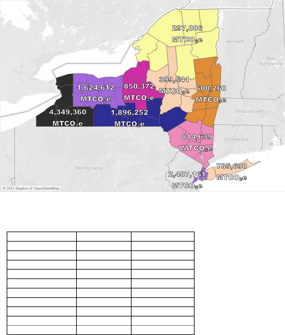
122
Figure 22. CH
4
Emissions by Economic Region in New York State in 2020 (AR5 GWP
20
)
Table 19. CH
4
Emissions by Economic Region in New York State in 2020
Upstate/Downstate
Region
% of CH
4
Emissions
Upstate
Western New York
30.8%
Upstate
Finger
Lakes
11.0%
Upstate
Southern
Tier
14.0%
Upstate
Central New York
6.0%
Upstate
North
Country
1.5%
Upstate
Mohawk Valley
3.4%
Upstate
Capital
District
4.3%
Downstate
Hudson
Valley
5.8%
Downstate
New York City
17.6%
Downstate
Long Island
5.6%
123
4.7 Summary
of
Source
Category
Comparison:
1990–2020
The largest upstream decrease in emissions was from conventional natural gas production from
high-producing wells (-89.3%), which follows the decreasing completion and production patterns
shown in Figure 2, Figure 4, and discussed in section 2. The midstream source categories saw increases
in emissions from transmission pipelines (+9.95%) due to increases in overall pipeline mileages in New
York State over that time period as well as large increases in CH
4
emissions from transmission (+8.5%)
and gas storage compressor stations (+52.9%), resulting from increases in the number of compressor
stations during that time period in order to accommodate increased pipeline capacity. Increases in
pipeline and storage capacity and associated compressors reflect trends toward increasing natural gas
consumption, as identified by EIA (2018). In the downstream source categories, there was a large
shift away from cast-iron and unprotected steel distribution mains toward lower emitting plastic pipes,
resulting in a net decrease in downstream emissions. Cast-iron and unprotected steel distribution mains
decreased by 59.1% and 54.8%, respectively, and plastic pipes increased by 292%. Although the plastic
distribution mains and services along with residential and commercial meter emissions have increased,
they were offset by larger reductions in emissions from replacing cast-iron and unprotected steel
pipelines (Figure 23).

124
Figure 23. Comparison of Source Category CH
4
Emissions from 1990 and 2020 in New York State, Using AR5 GWP
20
Conversion Factors
for CH
4

125
4.8
Emissions
Inventory
Validation
4.8.1 Comparison to the 2020 EPA GHG Inventory
The 2015 and prior versions of the New York State oil and natural gas sector methane emissions
inventory used a scaling approach to scale the national inventory to New York State based on the ratio
of national to State natural gas consumption. The current inventory applies a bottom-up, activity-driven
methodology to estimate emissions form the oil and natural gas sector. The updated and improved
methodology allows for direct comparison with other activity-based, bottom-up inventories, including
the 2020 EPA GHG Inventory (EPA 2022). The 2020 EPA GHG Inventory estimated total CH
4
emissions
from oil and natural gas systems to be 205.1 MMTCO
2
e in 2020. The NYS inventory finds total CH
4
emissions from the oil and natural gas sector to be 14.1 MMTCO
2
e in 2020 (AR5 GWP
20
), equivalent
to 6.87% of the total national inventory. Nationwide, EPA estimates a 15.7% decrease in emissions
since 1990 and a 0.24% decrease from 2005–2020, and the NYS inventory finds a 22.4% decrease since
1990, which is similar to the nationwide trend, and a 31.9% decrease from 2005–2020. Despite these
discrepancies, when viewing nationwide energy emissions trends described in the 2020 EPA GHG
Inventory (EPA 2022), the New York State time series CH
4
emissions follows the shape of the energy
sector emissions in the national inventory, shown in Figure 24. These data show a similar pattern to that
shown in Figure 12, growing to a peak in emissions in 2005 and subsequently declining. As such, patterns
in CH
4
emissions in New York State described here follow trends in large-scale nationwide energy shifts.
Figure 24. Reproduction of Figure ES-11 from (EPA 2022), Showing Time Series Trends in
Emissions from Energy and Other Sectors
126
4.8.2
Comparison
to Environmental Protection Agency’s Greenhouse Gas
Reporting Program Values
The EPA FLIGHT database shows Subpart W reported CH
4
emissions in NYS totaled 3.814 MMTCO
2
e
in 2020, while this inventory estimates a greater amount for the 2020 CH
4
emissions at 14.1 MMTCO
2
e.
One explanation for the discrepancy is that Subpart W reporting is required only for facilities emitting
more than 25,000 MTCO
2
e annually, whereas New York State has a large number of smaller facilities
that emit CH
4
, but do not reach the Subpart W reporting threshold. Most notably, Subpart W does not
require emissions from meters, pipelines, or buildings to be reported, and more specifically, Subpart W
data for 2020 show 3.57 MMTCO
2
e emitted by local distribution companies, 0.155 MMTCO
2
e from
transmission/compression, and 0.087 MMTCO
2
e from underground natural gas storage. This inventory
estimates emissions from natural gas distribution to be 4.34 MMTCO
2
e or 114% of emissions reported
under Subpart W—highlighting the importance of identifying proper distribution pipeline leak rates in
New York State to update EFs from national averages. The inventory shows that transmission compressor
stations are the largest single source category, with estimated emissions of 3.601 MMTCO
2
e in 2020,
indicating that total transmission compression emissions are underestimated by Subpart W. The inventory
estimates emissions from underground natural gas storage to be 1.85 MMTCO
2
e in 2020, which is an
order of magnitude greater than reported under Subpart W.
If downstream emissions are subtracted from the total inventory, upstream and midstream emissions
are estimated to be 8.94 MMTCO
2
e, which is 134% higher than emissions from these segments reported
under Subpart W in NYS. The discrepancy between emissions in Subpart W and the current inventory is
higher than the findings of Alvarez et al. (2018), who estimate CH
4
emissions from the oil and natural gas
supply chain to be ~ 60% greater than EPA estimates. As mentioned above, these discrepancies are the
result of facility reporting thresholds under Subpart W and missing methane emission sources. Again, this
discrepancy emphasizes the importance of detailed bottom-up inventories of all sources and the validation
of bottom-up inventories with top-down flight or satellite measurements.
4.8.3 Comparison to Other State Inventories
New York State is bordered by Pennsylvania, New Jersey, Connecticut, Massachusetts, and Vermont.
The following section provides a breakdown of the most recent inventory year for each of the adjacent
states. Pennsylvania primarily uses the default Environmental Protection Agency State Inventory
Tool (EPA SIT)tool to estimate emissions from the residential, commercial, industrial, transportation,
electricity production, agriculture, waste management, forestry, and land use sectors in Pennsylvania,
and uses AR4 GWP
100
values to report CO
2
equivalents.
20
Pennsylvania estimates total natural gas
127
and oil system emissions to be 12.33 MMTCO
2
e in 2020, largely governed by natural gas
production (8.11 MMTCO
2
e), natural gas transmission (2.07 MMTCO
2
e) and natural gas distribution
(2.09 MMTCO
2
e). As expected, Pennsylvania’s estimated emissions from the oil and natural gas sector
are much higher than in New York State, when converted to AR5 GWP
20
estimates. Pennsylvania is the
second largest producer of natural gas in the United States, second only to Texas and produced about
7.148 million Mcf of natural gas in 2020, compared with 9,692 Mcf in New York State in 2020. New
York State had 49 well completions in 2020, compared to Pennsylvania’s 476 unconventional and
51 conventional wells drilled.
21
New Jersey derives 55% of electricity generation from natural gas and has seen a total of 36 exploration
wells drilled, none of which were drilled after 1982, due to a lack of natural gas resources and regulations.
As such, New Jersey is primarily a consumer of natural gas, as identified by the 2020 GHG inventory,
22
which estimates emissions of 2.3 MMTCO
2
e from the natural gas transmission and distribution segments.
New Jersey employs the EPA SIT to estimate emissions from natural gas transmission and
distribution segments.
Connecticut relies heavily on the EPA SIT to calculate GHG emissions by sector. Connecticut is
primarily a natural gas consuming state, as they have minimal oil and natural gas resources. Based
on review of the 2018 inventory
23
and supporting data, Connecticut does not explicitly estimate
emissions from the oil and natural gas sector, instead emissions are reported for the Agriculture,
Commercial, Electric Power (consumption), Industrial, Residential, Transportation, and Waste sectors.
Total emissions in Connecticut in 2020 were estimated to be 42.2 to 43.7 MMTCO
2
e depending on
whether emission estimates were based on electric consumption or generation. Given the aggregated
nature of the Connecticut GHG inventory, it is challenging to draw direct comparisons to the New
York State inventory.
Massachusetts identifies only the transmission and distribution segments of the oil and natural gas
sector as relevant to Massachusetts, using the EPA SIT to estimate emissions from leaks in pipelines
and services, customer meters, and metering/regulating stations and venting. Estimated emissions from
natural gas transmission and distribution systems in 2016,
24
the most recent year of complete data,
were 0.8 MMTCO
2
e.

128
Vermont’s GHG Inventory
25
uses the EPA SIT along with methodologies developed by the Vermont
Agency of Natural Resources, Vermont Department of Public Service and the Center for Climate
Strategies. Vermont has no upstream production of oil or natural gas, and midstream and downstream
emissions estimates are very small, reflecting low consumption of natural gas in the state (11,926 MMcf
in 2020) compared with New York State (1,263,584 MMcf in 2020). Vermont estimates total emissions
from the midstream and downstream segments of the oil and natural gas sector to be 0.03 MMTCO
2
e.
A comparison of the New York State inventory with each of the discussed state inventories is shown in
Table 20. As shown, the ratio of estimated emissions to consumption is consistent for most states, with
the exception of Pennsylvania and Vermont, which both have very different natural gas profiles than the
other states. Pennsylvania has much higher upstream production of natural gas, resulting in a much higher
ratio of emissions to consumption, as emissions associated with production increase the ratio. Vermont
has minimal natural gas infrastructure and very low consumption, resulting in a ratio of emissions to
consumption that is an order of magnitude lower than the other states in the region.
Table 20. Comparison of This Inventory to the Most Recent Year of Adjacent State Inventories
NYS
(AR5
GWP20)
Pennsylvania
(AR4 GWP100)
New Jersey
(AR4
GWP100)
Connecticut
Massachusetts
(AR4 GWP100)
Vermont
(AR4
GWP100)
Year
2020
2019
2019
2018
2016
2017
Oil and Gas CH
4
(MMTCO
2
e)
14.1
12.33
2.3
*
0.8
0.03
Consumption
(MMcf)
1,263,584
1,618,008
761,005
277,931
427,946
11,926
Production
(MMcf)
9,692
7,148,295
0
0
0
0
Emissions/
consumption
2.12x10
-06
8.57x10
-06
2.95x10
-06
N/A
1.87x10
-06
0.42x10
-06
*
Connecticut data are not broken out for the oil and natural gas sector.
Note: Consumption and production are derived from EIA data for the year of the inventory.
4.8.4 Comparison to Top-Down and Bottom-Up Studies
Validation of an emission inventory using alternate methodologies is an important step in determining
the robustness of the inventory. The NYS inventory uses a bottom-up methodology to estimate emissions
using site-level activity data and EFs. Recent efforts in the literature have shown discrepancies between
bottom-up and top-down methodology (see e.g., Marchese et al. 2015; Mitchell et al. 2015; Omara,
Sullivan, Li, Subramanian, et al. 2016; Subramanian et al. 2015; Alvarez et al. 2018). One of the
129
challenges with validating bottom-up emission inventories with top-down studies is the availability
of top-down study data. As discussed in section 3.1.2.6, top-down studies require detailed atmospheric
measurements and modeling to estimate emission flux. Thorough review of the available literature,
and consultation with the Project Advisory Committee (PAC) and other experts during the first phase,
revealed a lack of available top-down data specific to New York State. As identified throughout the
discussion of EFs in section 3, it will be beneficial for the State to validate that the EFs applied accurately
reflect local conditions. Top-down studies can provide validation of local conditions, but only at the site
and regional level, and therefore, New York State should consider top-down validation of the higher
emitting segments of the inventory. Such validation could potentially reduce the uncertainty in
the inventory.
4.9 Uncertainty
Uncertainty is widely addressed in section 3 in a discussion about uncertainty in relation to the limitations
of the EFs used. Although best practices are followed and EFs are employed from a number of EPA tools,
several sources have been identified that warrant discussion.
First, emissions from gathering, transmission, and distribution pipelines comprise a large fraction of the
total emissions estimated in this inventory. The literature on emission rates from pipelines is not deep,
with most studies focusing specifically on certain cities. Therefore, the EFs used are based on guidance
from the EPA Oil and Gas Tool and EPA’s SIT; however, upon inspection, many of those EFs are
derived from older studies that were performed in other states. As such, there is a research need to
produce new empirical data on per-mile leak rates that better reflect present conditions in New
York State.
Second, transmission and storage compressor stations have been identified as large sources of CH
4
in
the State. The emission estimation methodology applies an EF based on peer-reviewed literature, which
employs best practices to measure and estimate emissions from compressors. However, those studies,
along with others, identify a potentially wide range of emission rates from compressor stations under
normal operating conditions, with a non-normal distribution. Therefore, applying a central estimate
to estimate emissions inherently introduces uncertainty into the estimate.
130
Third, this inventory is based on the best available activity data and EFs. However, given data limitations,
this inventory is limited to site-level estimates, as component counts are unavailable for New York State
facilities. As such, State facilities may have different component compositions to those applied in this
inventory, resulting in the possible application of EFs that could be better tailored to New York State.
Fourth, emissions from high-emitting sources are not explicitly estimated. High-emitting sources have
been widely observed and described in the literature along all stages of the upstream, midstream, and
downstream process, with a small number of sites or facilities contributing a majority of regional
emissions in many instances. However, given the unknown distribution of high-emitting sources in the
State, it is challenging to apply statistical methods to estimate the likelihood of high-emitting sources.
4.9.1 Emission Inventory Uncertainty
Using the uncertainty bounds identified in Table 6, the following figures present the total time series
emissions including upper and lower confidence bounds. Comparing Figure 25 and Figure 27 the lower
bound on the uncertainty estimate is driven by midstream emissions. It was determined that selecting the
lower-bound value represented the most applicable value to New York State, and so the best estimate
and the lower-bound estimate are the same for the upstream and downstream emissions factors.
Upper-bound emissions estimates were determined by selecting the upper bound EF provided by
the sources chosen for the best estimate EFs. As such, upper-bound emission estimates may be thought
of as representing the upper limit of emissions for the State, based on EFs from other states which
employ high-emitting techniques in the oil and natural gas sector. These upper-bound estimates also
reflect literature estimates of EFs for many source categories with identified high-emitting sources, as
discussed in section 3. As such, these EFs also likely capture the possible range of uncertainty that arises
from accounting for high-emitting sources in the State, which is especially notable in the upstream and
downstream source categories. In the upstream and downstream source categories, the upper-bound
emission estimates are four and two times the best estimate values, respectively, reflecting the wide
range of uncertainty that arises from incorporating EFs that are derived with high-emitting sources
in the sample population.

131
Figure 25. Total Emissions Including Best Estimate and Upper and Lower Bounds (AR5 GWP
20
)
Figure 26. Upstream Emissions Including Upper and Lower Bounds (AR5 GWP
20
)
Figure 27. Midstream Emissions Including Upper and Lower Bounds (AR5 GWP
20
)

132
Figure 28. Downstream Emissions Including Upper and Lower Bounds (AR5 GWP
20
)
4.10
Comparing
AR4
and
AR5
Emission
Estimates
Methane is a short-lived climate pollutant, with a lifetime of approximately 12 years. In order to
capture the near-term climate impacts of methane emissions most effectively, results are reported in
terms of AR5 GWP
20
. However, these results, along with discussion in appendix A.5, show that reporting
emissions using a range of GWPs, including AR4, AR5, and both short-term and long-term climate
effects, can provide a more comprehensive illustration of climate impact. Selection of alternate GWPs
depending on AR4 or AR5, and short-term or long-term climate effects, can yield markedly different
results. Recent literature has indicated that it is important to consider the short-lived effects of CH
4
,
described by the GWP
20
. The CH
4
emissions estimates presented throughout this report are the AR5
GWP
20
estimates. Under AR4, GWP
100
for CH
4
is 25, and GWP
20
is 72. AR4 estimates from 2007
were updated in 2014 in IPCC’s AR5, which increased the GWP
100
to 28, and GWP
20
to 84. Under AR6,
GWP
20
was decreased to 82.5 for fossil origin CH
4
and 80.8 for non-fossil origin CH
4
while GWP
100
was
changed to 29.8 for fossil CH
4
and 27.2 for non-fossil CH
4
(IPCC 2021). The following section describes
the 2020 emissions estimated in the context of both AR4 and AR5 GWPs and the statewide inventory.
As shown in Table 21, simply changing the GWP from AR4 GWP
100
to GWP
20
for the original, 2015
New York State inventory increases CH
4
emissions from 2.22 MMTCO
2
e to 6.39 MMTCO
2
e for the oil
and natural gas sector. Under AR5 GWP
100
, this inventory finds CO
2
e emissions are 11.9% higher than
estimates under AR4 GWP
100
. Under AR5 GWP
20
, emissions estimates are16.6% higher than estimates
under AR4 GWP
20
.

133
Table 21. Comparison of AR4 and AR5 GWP
100
and GWP
20
Values Applied to the 2020 Oil and Gas
Systems CH
4
Emissions in New York State (MMTCO
2
e)
AR4 GWP
100
AR4 GWP
20
AR5
GWP
100
AR5 GWP
20
CH
4
GWP (CO
2
e)
25
72
28
84
N
2O GWP (CO
2
e)
298
289
265
264
NYSERDA 2015
Inventory
Oil
and Gas CH
4
(MMTCO
2
e)
2.22
6.39
2.49
7.46
Current Inventory
2017 Oil and Gas CH
4
(MMTCO
2
e)
2.66 7.67 2.98 8.95
2020
Oil and Gas CH
4
(MMTCO
2
e)
4.20
12.09
4.70
14.10

134
5 Future Improvements
Emissions inventory development is a continuous process that requires making improvements as better
data on emission factors and emission source activity become available. In addition, measurements of
atmospheric methane concentration can be used to assess the completeness/accuracy of the emissions
inventory. Below is a list of actions that NYS is currently taking to potentially improve future inventories:
• Continuing to review literature to identify new data on emissions factors and emission
source activity.
• Identifying additional sources of methane emissions to include in the NYS oil and natural
gas sector methane emissions inventory such as:
o Residential refrigeration and clothes dryers.
o Commercial buildings beyond restaurants and hospitals. Currently, data on methane leaks
in other commercial buildings is lacking. The inventory does not currently use the data from
restaurants and hospitals as a surrogate for other commercial buildings because it is thought
that restaurants and hospitals will have a different emissions profile than office buildings
and other commercial buildings. To understand the potential missing emissions, applying
the average hospital/restaurant emissions factor to all other commercial buildings results in
emissions of around 1 million MTCO
2
e (AR5, GWP
20
) or roughly 8% of the current 2020
inventory, which is likely an overestimate.
o Industrial buildings.
• Investigating the impacts of cast iron pipeline reconditioning on emissions estimates from
existing cast iron pipeline infrastructure.
• Assessing whether NYS’s usage of a higher natural gas odorant concentration results in a larger
number of leak detection and repairs in buildings, and therefore lower emissions, than states
that require lower odorant concentrations.
• As data become available, comparing top-down measurements of methane emissions to the
bottom-up inventory values to verify inventory and identify further areas for
potential improvement.

135
6 Conclusions
With the passage of the Climate Leadership and Community Protection Act in 2019, New York State
has committed to reduce economy-wide greenhouse gas emissions 40% by 2030 and no less than
85% by 2050 from 1990 levels. While efforts to date have focused on the reduction of carbon dioxide
(CO
2
) emissions—the dominant cause of the rise in global average temperature—New York State is
turning its attention to methane due to its significant short-term impacts on climate change. The goal
of this project is to support CH
4
emission reduction efforts in New York State, and achievement of the
Climate Act goals, by improving the State’s understanding of CH
4
emissions from the oil and natural
gas sector.
Based on the four identified areas of best practices and recommendations developed under the first
phase of the project (described in appendix A and presented in the following table and discussion),
this inventory presents a marked improvement compared to prior iterations of the New York State oil
and natural gas sector methane emission inventories. Emissions inventory development is a continuous
process that requires making improvements as better data on emissions factors and emission source
activity become available. In each phase of this product, the inventory has improved as up-to-date
data on activity and emissions factors are identified. NYS is taking additional steps to improve
future inventories. Table 22 summarizes the best practice recommendations, implementation of these
recommendations when developing the current inventory and areas for future inventory improvement.
Table 22. Summary of Best Practice Recommendations, Implementation of Best Practices and
Areas for Future Inventory Improvements
Recommendation
#1
New York State should develop a more detailed set of activity data,
including
site
- and component-level data, for its CH
4
inventory in order to create an inventory with the detail
need
ed to capture the impacts of CH
4
mitigation strategies targeted at the site- or component-level.
Implementation in Current
Inventory:
Applied the best available activity data, using publicly
available inputs as
well as data provided by New York State agencies.
Areas
for Future Improvement:
• Collect/compile data on the number and location of transmission and storage compressor
stations in the State, including stations that only have electric compressors.
• Collect/compile data on the county-level miles of distribution pipeline by pipeline material.
• Collect/compile data on the county-level number of residential and commercial/industrial
gas
meters.
•
Identify additional sources of methane emissions to include in the inventory and
collect/compile data on county-level activity.

136
Table 22 continued
Recommendation
#2
New York State should estimate and apply EFs for upstream and
downstream oil and gas activities in the
State using best available data, validated by both bottom-
up and top
-down studies, and specific to geographic location.
Implementation in Current Inventory:
Applied the best available EFs from the published literature.
Areas
for Future Improvement:
• Develop New York State-specific EFs for well pads during production.
• Develop New York State-specific EFs for transmission and storage compressor stations.
• Develop an EF
for fugitive emissions from storage reservoirs.
• Identify EFs for other types of commercial buildings, industrial buildings, and additional residential
appliances.
Recommendation
#3
New York State should align available geospatial data with inventory data
as
much as possible to create a geospatial emissions inventory that allows greater consideration
of
identifying
hot spots and air quality concerns as well as verification of emission inventories with
empirical
data.
Implementation in Current
Inventory:
Results are presented geospatially, allocated to the
county
-level, with the ability to produce sub-county results for many segments.
Areas
for Future Improvement:
• Collect air quality data on ambient CH
4
concentrations throughout New York State
and use the
observed concentrations to verify emission estimates.
• As data become available, compare top-down measurements of methane emissions to the
inventory to verify inventory and identify areas for potential improvement.
Recommendation
#4
New York State should conduct uncertainty analysis when calculating and
reporting
its CH
4
inventory. At a minimum, that uncertainty analysis should account for uncertainties
in
published EFs, but it could also include an assessment of high-emitting sources across the State.
New
York State should develop and apply models that help account for the existence of high-emitting
sources either in cases where emission releases are known (e.g., reported leakage) or in cases where
emission releases are
not known (e.g., estimated leakage based on pipeline age or material).
Implementation in Current
Inventory:
Assessed uncertainty in the applied EFs to identify the
most likely range
of CH
4
emission from the oil and natural gas sector. With better information on
the
statistical
distribution of high-emitting sources, this inventory methodology may also be applied
to
explicitly
include high
-emitting sources.
Areas
for Future Improvement:
• Develop a better understanding of the distribution of high-emitting sources and the frequency
of
operation in the high-emitting state.
I
n the current inventory, total CH
4
emissions in 2020 were estimated to be 14.105 MMTCO
2
e (AR5,
GWP
20
), and estimates for 2020 were equivalent to 6.87% of the total nationwide emissions estimated
by EPA. Largely driven by decreases in high-producing well activity—and a transition away from more
leak-prone cast-iron and unprotected steel pipelines to plastic—results from this inventory show that,
despite an increase in natural gas consumption, total CH
4
emissions have continued to decline since
2005, with an average annual decrease of 1.06% per year. Decreasing emissions agrees with observed
large-scale nationwide energy shifts. The largest methane emission source categories identified in the
137
State inventory developed under this project include transmission compressor stations, low producing
conventional gas wells, natural gas storage compressor stations, cast iron distribution pipeline mains,
unprotected steel distribution pipeline mains, unprotected steel distribution pipeline services, and high
producing conventional gas wells.
The current inventory being presented builds off the methodology developed for the 2017 inventory and
incorporates findings from the most current empirical research. By continuing to apply established best
practices based on a thorough review of the literature and expert consultation, the inventory improves
the methane emissions baseline in New York State.

138
7 References
Allen, David T. 2014. “Methane Emissions from Natural Gas Production and Use: Reconciling Bottom-
up and Top-down Measurements.” Current Opinion in Chemical Engineering 5. Elsevier Ltd: 78-83.
https://doi.org/10.1016/j.coche.2014.05.004
———. 2016. “Emissions from Oil and Gas Operations in the United States and Their Air Quality
Implications.” Journal of the Air & Waste Management Association 66 (6). Taylor & Francis:
549-75. https://doi.org/10.1080/10962247.2016.1171263
Allen, David T., Adam P. Pacsi, David W. Sullivan, Daniel Zavala-Araiza, Matthew Harrison, Kindal
Keen, Matthew P. Fraser, A. Daniel Hill, Robert F. Sawyer, and John H. Seinfeld. 2015. “Methane
Emissions from Process Equipment at Natural Gas Production Sites in the United States: Pneumatic
Controllers.” Environmental Science and Technology 49 (1): 633-40.
https://doi.org/10.1021/es5040156
Allen, David T., David W. Sullivan, Daniel Zavala-Araiza, Adam P. Pacsi, Matthew Harrison, Kindal
Keen, Matthew P. Fraser, et al. 2015. “Methane Emissions from Process Equipment at Natural Gas
Production Sites in the United States: Liquid Unloadings.” Environmental Science & Technology
49(1): 641-48. https://doi.org/10.1021/es504016r
Allen, David T, Vincent M Torres, James Thomas, David W Sullivan, Matthew Harrison, Al Hendler,
Scott C Herndon, et al. 2013. “Measurements of Methane Emissions at Natural Gas Production Sites
in the United States.” Proceedings of the National Academy of Sciences of the United States of
America 110 (44). National Academy of Sciences: 17768-73.
https://doi.org/10.1073/pnas.1304880110
Alvarez, R.A., David R. Lyon, Anthony J. Marchese, Allen L. Robinson, and Steven P. Hamburg. 2016.
“Possible Malfunction in Widely Used Methane Sampler Deserves Attention but Poses Limited
Implications for Supply Chain Emission Estimates.” Elementa: Science of the Anthropocene 4:
000137. https://doi.org/10.12952/journal.elementa.000137
Alvarez, R.A., S.W. Pacala, J.J. Winebrake, W.L. Chameides, and S.P. Hamburg. 2012. “Greater Focus
Needed on Methane Leakage from Natural Gas Infrastructure.” Proceedings of the National Academy
of Sciences of the United States of America 109 (17). https://doi.org/10.1073/pnas.1202407109
Alvarez, R.A., Daniel Zavala-araiza, David R Lyon, David T Allen, Zachary R Barkley, R Adam,
Kenneth J Davis, et al. 2018. “Assessment of Methane Emissions from the U.S. Oil and Gas Supply
Chain.” Science 7204 (June): 1-9. https://doi.org/10.1126/science.aar7204
Balcombe, Paul, Jamie F Speirs, Nigel Brandon, and Adam Hawkes. 2018. “Methane Emissions:
Choosing the Right Climate Metric and Time Horizon.” Environmental Science: Processes &
Impacts. The Royal Society of Chemistry. https://doi.org/10.1039/C8EM00414E
139
Barkley, Zachary R., Thomas Lauvaux, Kenneth J. Davis, Aijun Deng, Natasha L. Miles, Scott J.
Richardson, Yanni Cao, et al. 2017. “Quantifying Methane Emissions from Natural Gas Production
in North-Eastern Pennsylvania.” Atmospheric Chemistry and Physics 17 (22): 13941-66.
https://doi.org/10.5194/acp-17-13941-2017
Blackhurst, Michael, H. Scott Matthews, Aurora L. Sharrard, Chris T. Hendrickson, and Ins Lima
Azevedo. 2011. “Preparing US Community Greenhouse Gas Inventories for Climate Action Plans.”
Environmental Research Letters 6 (3). https://doi.org/10.1088/1748-9326/6/3/034003
Brandt, A R, G A Heath, E A Kort, F O’Sullivan, G Petron, S M Jordaan, P Tans, et al. 2014. “Energy
and Environment. Methane Leaks from North American Natural Gas Systems.” Science (New York,
N.Y.) 343 (6172). United States: 733-35. https://doi.org/10.1126/science.1247045
Brandt, Adam R, Garvin A Heath, and Daniel Cooley. 2016. “Methane Leaks from Natural Gas Systems
Follow Extreme Distributions.” Environmental Science & Technology 50 (22). American Chemical
Society: 12512-20. https://doi.org/10.1021/acs.est.6b04303
Brantley, Halley L., Eben D. Thoma, William C. Squier, Birnur B. Guven, and David Lyon. 2014.
“Assessment of Methane Emissions from Oil and Gas Production Pads Using Mobile
Measurements.” Environmental Science and Technology 48 (24): 14508-15.
https://doi.org/10.1021/es503070q
Burnham, Andrew, Jeongwoo Han, Corrie E Clark, Michael Wang, Jennifer B Dunn, and Ignasi Palou-
Rivera. 2012. “Life-Cycle Greenhouse Gas Emissions of Shale Gas, Natural Gas, Coal, and
Petroleum.” Environmental Science & Technology 46 (2). American Chemical Society: 619-27.
https://doi.org/10.1021/es201942m
Cathles, Lawrence M., Larry Brown, Milton Taam, and Andrew Hunter. 2012. “A Commentary on ‘The
Greenhouse-Gas Footprint of Natural Gas in Shale Formations’ by R.W. Howarth, R. Santoro, and
Anthony Ingraffea.” Climatic Change 113 (2): 525-35. https://doi.org/10.1007/s10584-011-0333-0
Caulton, D. R., P. B. Shepson, R. L. Santoro, J. P. Sparks, R. W. Howarth, A. R. Ingraffea, M. O. L.
Cambaliza, et al. 2014. “Toward a Better Understanding and Quantification of Methane Emissions
from Shale Gas Development.” Proceedings of the National Academy of Sciences 111 (17): 6237-42.
https://doi.org/10.1073/pnas.1316546111
CenSARA. 2012. “2011 Oil and Gas Emission Inventory Enhancement Project for CenSARA States.”
https://www.arb.ca.gov/ei/areasrc/oilandgaseifinalreport.pdf
Clark, Nigel N, David L McKain, Derek R Johnson, W Scott Wayne, Hailin Li, Vyacheslav Akkerman,
Cesar Sandoval, et al. 2017. “Pump-to-Wheels Methane Emissions from the Heavy-Duty
Transportation Sector.” Environmental Science & Technology 51 (2). American Chemical Society:
968-76. https://doi.org/10.1021/acs.est.5b06059
Clearstone. 2011. “Clearstone Engineering, Development of Updated Emission Factors for Residential
Meters.”
140
Conley, S, G Franco, I Faloona, D R Blake, J Peischl, and T B Ryerson. 2016. “Methane Emissions from
the 2015 Aliso Canyon Blowout in Los Angeles, CA.” Science 351 (6279): 1317 LP-1320.
http://science.sciencemag.org/content/351/6279/1317.abstract
EDF. 2018. “Methane Research Series: 16 Studies.” 2018. https://www.edf.org/climate/methane-research-
series-16-studies
EIA. 2018a. “New York Natural Gas Total Consumption.” 2018.
https://www.eia.gov/dnav/ng/hist/na1490_sny_2a.htm
EIA. 2018b. Residential Energy Consumption Survey (RECS). 2015 RECS Survey Data.
https://www.eia.gov/consumption/residential/data/2015/
EIA. 2019. Natural gas explained - Use of natural gas. https://www.eia.gov/energyexplained/natural-
gas/use-of-natural-gas.php
EIA. 2021. “New York Natural Gas Total Consumption.” 2021.
https://www.eia.gov/dnav/ng/hist/na1490_sny_2a.htm
Empire State Organized Geologic Information System (ESOGIS). 2021. All Wells – ZIP File.
https://esogis.nysm.nysed.gov/
Etminan, M., G. Myhre, E. J. Highwood, and K. P. Shine. 2016. “Radiative Forcing of Carbon Dioxide,
Methane, and Nitrous Oxide: A Significant Revision of the Methane Radiative Forcing.” Geophysical
Research Letters. https://doi.org/10.1002/2016GL071930
European Environment Agency. 2018. “Annual European Union Greenhouse Gas Inventory 1990-2016
and Inventory Report 2018.” https://www.eea.europa.eu/publications/european-union-greenhouse-
gas-inventory-2018
Fischer, Joseph C. Von, Daniel Cooley, Sam Chamberlain, Adam Gaylord, Claire J. Griebenow, Steven P.
Hamburg, Jessica Salo, Russ Schumacher, David Theobald, and Jay Ham. 2017. “Rapid, Vehicle-
Based Identification of Location and Magnitude of Urban Natural Gas Pipeline Leaks.”
Environmental Science and Technology 51 (7): 4091-99. https://doi.org/10.1021/acs.est.6b06095
Fischer, M.L., Chan, W.R., Delp, W., Jeong, S. et al. 2018a. An estimate of natural gas methane
emissions from California homes. Environmental Science & Technology 52(17): 10205-10213.
https://doi.org/10.1021/acs.est.8b03217
Fischer, M.L., Chan, W.R., Delp, W., Jeong, S. et al. 2018b. Supplementary material. An estimate of
natural gas methane emissions from California homes. Environmental Science & Technology 52(17):
10205-10213.
https://pubs.acs.org/doi/suppl/10.1021/acs.est.8b03217/suppl_file/es8b03217_si_001.pdf
Frankenberg, Christian, Andrew K. Thorpe, David R. Thompson, Glynn Hulley, Eric Adam Kort, Nick
Vance, Jakob Borchardt, et al. 2016. “Airborne Methane Remote Measurements Reveal Heavy-Tail
Flux Distribution in Four Corners Region.” Proceedings of the National Academy of Sciences
113(35): 9734-39. https://doi.org/10.1073/pnas.1605617113
141
GTI. 2009. “Field Measurement Program to Improve Uncertainties for Key Greenhouse Gas Emission
Factors for Distribution Sources. GTI Project Number 20497. OTD Project Number 7.7.B”
Harrison, M.R., Tm Shires, Jk Wessels, and Rm Cowgill. 1997a. “Methane Emissions from the Natural
Gas Industry.” Epa and Wma Annual Meeting 7: 93. http://p2pays.net/ref/07/06348.pdf
———. 1997b. “Methane Emissions from the Natural Gas Industry.” EPA and WMA Annual
Meeting 7: 93
Harriss, Robert, Ramón A Alvarez, David Lyon, Daniel Zavala-Araiza, Drew Nelson, and Steven P
Hamburg. 2015. “Using Multi-Scale Measurements to Improve Methane Emission Estimates from Oil
and Gas Operations in the Barnett Shale Region, Texas.” Environmental Science & Technology 49
(13). American Chemical Society: 7524-26. https://doi.org/10.1021/acs.est.5b02305
Hartmann, D. L., a. M. G. K. Tank, and M. Rusticucci. 2013. “IPCC Fifth Assessment Report, Climatie
Change 2013: The Physical Science Basis.” IPCC AR5 (January 2014): 31-39
Hayhoe, Katharine, Haroon S Kheshgi, Atul K Jain, and Donald J Wuebbles. 2002. “Substitution of
Natural Gas for Coal: Climatic Effects of Utility Sector Emissions.” Climatic Change 54 (1): 107-39.
https://doi.org/10.1023/A:1015737505552
Heath, Garvin, Ethan Warner, Daniel Steinberg, and Adam Brandt. 2015. “Estimating U.S. Methane
Emissions from the Natural Gas Supply Chain. Approaches, Uncertainties, Current Estimates, and Future
Studies,” no. August. https://doi.org/10.2172/1226158
Hendrick, Margaret F., Robert Ackley, Bahare Sanaie-Movahed, Xiaojing Tang, and Nathan G. Phillips.
2016. “Fugitive Methane Emissions from Leak-Prone Natural Gas Distribution Infrastructure in Urban
Environments.” Environmental Pollution 213. Elsevier Ltd: 710-16.
https://doi.org/10.1016/j.envpol.2016.01.094
Hong, B. & Howarth, R.W. 2016. Greenhouse gas emissions from domestic hot water: heat pumps
compared to most commonly used systems. Energy Science & Engineering 4(2): 123-133.
https://doi.org/10.1002/ese3.112
Howarth, Robert W. 2014. “A Bridge to Nowhere: Methane Emissions and the Greenhouse Gas Footprint
of Natural Gas.” Energy Science & Engineering 2 (2): 47-60. https://doi.org/10.1002/ese3.35.
Howarth, Robert W., Renee Santoro, and Anthony Ingraffea. 2011. “Methane and the Greenhouse-Gas
Footprint of Natural Gas from Shale Formations.” Climatic Change 106 (4): 679-90.
https://doi.org/10.1007/s10584-011-0061-5
Hultman, Nathan, Dylan Rebois, Michael Scholten, and Christopher Ramig. 2011. “Erratum: The
Greenhouse Impact of Unconventional Gas for Electricity Generation (Environmental Research
Letters (2011) 6 (044008)).” Environmental Research Letters 6 (4). https://doi.org/10.1088/1748-
9326/6/4/049504
IPCC. 2006. “2006 IPCC Guidelines for National Greenhouse Gas Inventories.” Vol. 2.
142
IPCC. 2021. IPCC Sixth Assessment Report, Climate Change 2021: The Physical Science Basis.”
https://www.ipcc.ch/report/ar6/wg1/
ITRC. 2018. “Evaluation of Innovative Methane Detection Technologies: Appendix B –
Characterization.” Washington, D.C
Jaramillo, Paulina, W Michael Griffin, and H Scott Matthews. 2007. “Comparative Life-Cycle Air
Emissions of Coal, Domestic Natural Gas, LNG, and SNG for Electricity Generation.” Environmental
Science & Technology 41 (17). American Chemical Society: 6290-96.
https://doi.org/10.1021/es063031o
Jiang, Mohan, W. Michael Griffin, Chris Hendrickson, Paulina Jaramillo, Jeanne Vanbriesen, and Aranya
Venkatesh. 2011. “Life Cycle Greenhouse Gas Emissions of Marcellus Shale Gas.” Environmental
Research Letters 6 (3). https://doi.org/10.1088/1748-9326/6/3/034014
Johnson, D, A Covington, and N Clark. 2015. “Methane Emissions from Leak and Loss Audits of Natural
Gas Compressor Stations and Storage Facilities.” Environmental Science and Technology 49 (13):
8132–8138. https://doi.org/10.1021/es506163m
Kang, Mary, Cynthia M. Kanno, Matthew C. Reid, Xin Zhang, Denise L. Mauzerall, Michael A. Celia,
Yuheng Chen, and Tullis C. Onstott. 2014. “Direct Measurements of Methane Emissions from
Abandoned Oil and Gas Wells in Pennsylvania.” Proceedings of the National Academy of Sciences
111 (51): 18173-77. https://doi.org/10.1073/pnas.1408315111
Karion, A., Colm Sweeney, Gabrielle Pétron, Gregory Frost, R. Michael Hardesty, Jonathan Kofler, Ben
R. Miller, et al. 2013. “Methane Emissions Estimate from Airborne Measurements over a Western
United States Natural Gas Field.” Geophysical Research Letters 40 (16): 4393-97.
https://doi.org/10.1002/grl.50811
Karion, A, C Sweeney, E A Kort, P B Shepson, A Brewer, M O L Cambaliza, S Conley, K J Davis, A
Deng, and M Hardesty. 2015. “Aircraft-Based Estimate of Total Methane Emissions from the Barnett
Shale Region.” Environmental Science and Technology 49 (13): 8124–8131
https://doi.org/10.1021/acs.est.5b00217
Karion, Anna, Colm Sweeney, Gabrielle Pétron, Gregory Frost, R. Michael Hardesty, Jonathan Kofler,
Ben R. Miller, et al. 2013. “Methane Emissions Estimate from Airborne Measurements over a
Western United States Natural Gas Field.” Geophysical Research Letters 40 (16): 4393-97.
https://doi.org/10.1002/grl.50811
Kirchgessner, D. 1997. “Estimate of Methane Emissions from the U.S. Natural Gas Industry.”
Chemosphere 35: 1365-90. https://doi.org/10.1016/S0045-6535(97)00236-1
Lamb, Brian K., Steven L. Edburg, Thomas W. Ferrara, Touché Howard, Matthew R. Harrison, Charles E.
Kolb, Amy Townsend-Small, Wesley Dyck, Antonio Possolo, and James R. Whetstone. 2015. “Direct
Measurements Show Decreasing Methane Emissions from Natural Gas Local Distribution Systems in
the United States.” Environmental Science and Technology 49 (8): 5161-69.
https://doi.org/10.1021/es505116p
143
Lavoie, T N, P B Shepson, M O L Cambaliza, B H Stirm, A Karion, C Sweeney, T I Yacovitch, S C
Herndon, X Lan, and D Lyon. 2015. “Aircraft-Based Measurements of Point Source Methane
Emissions in the Barnett Shale Basin.” Environmental Science and Technology 49 (13): 7904–7913.
https://doi.org/10.1021/acs.est.5b00410
Lebel, E.D., Lu, H.S., Speizer, S.A., Finnegan, C.J. et al. 2020. Quantifying methane emissions from
natural gas water heaters. Environmental Science & Technology.
https://doi.org/10.1021/acs.est.9b07189
Littlefield, James A., Joe Marriott, Greg A. Schivley, and Timothy J. Skone. 2017. “Synthesis of Recent
Ground-Level Methane Emission Measurements from the U.S. Natural Gas Supply Chain.” Journal of
Cleaner Production 148: 118-26. https://doi.org/10.1016/j.jclepro.2017.01.101
Lyon, David R., Ramón A. Alvarez, Daniel Zavala-Araiza, Adam R. Brandt, Robert B. Jackson, and
Steven P. Hamburg. 2016. “Aerial Surveys of Elevated Hydrocarbon Emissions from Oil and Gas
Production Sites.” Environmental Science and Technology 50 (9): 4877-86.
https://doi.org/10.1021/acs.est.6b00705
Lyon, David R., Daniel Zavala-Araiza, Ramón A. Alvarez, Robert Harriss, Virginia Palacios, Xin Lan,
Robert Talbot, et al. 2015. “Constructing a Spatially Resolved Methane Emission Inventory for the
Barnett Shale Region.” Environmental Science and Technology 49 (13): 8147-57.
https://doi.org/10.1021/es506359c
Marchese, Anthony J., Timothy L. Vaughn, Daniel J. Zimmerle, David M. Martinez, Laurie L. Williams,
Allen L. Robinson, Austin L. Mitchell, et al. 2015. “Methane Emissions from United States Natural
Gas Gathering and Processing.” Environmental Science and Technology 49 (17): 10718-27.
https://doi.org/10.1021/acs.est.5b02275
McKain, Kathryn, Adrian Down, Steve M. Raciti, John Budney, Lucy R. Hutyra, Cody Floerchinger,
Scott C. Herndon, et al. 2015. “Methane Emissions from Natural Gas Infrastructure and Use in the
Urban Region of Boston, Massachusetts.” Proceedings of the National Academy of Sciences 112 (7):
1941-46. https://doi.org/10.1073/pnas.1416261112
Merrin, Z. & Francisco, P.W. 2019. Unburned methane emissions from residential natural gas appliances.
Environmental Science & Technology 53: 5473-5482. https://doi.org/10.1021/acs.est.8b05323
Miller, S. M., S. C. Wofsy, A. M. Michalak, E. A. Kort, A. E. Andrews, S. C. Biraud, E. J. Dlugokencky,
et al. 2013. “Anthropogenic Emissions of Methane in the United States.” Proceedings of the National
Academy of Sciences. https://doi.org/10.1073/pnas.1314392110
Mitchell, Austin L, Daniel S Tkacik, Joseph R Roscioli, Scott C Herndon, Tara I Yacovitch, David M
Martinez, Timothy L Vaughn, et al. 2015. “Measurements of Methane Emissions from Natural Gas
Gathering Facilities and Processing Plants: Measurement Results.” Environmental Science &
Technology 49 (5). American Chemical Society: 3219-27. https://doi.org/10.1021/es5052809
144
Moore C, Stuver S, Kristine W. 2019. Classification of Methane Emissions from Industrial Meters,
Vintage versus Modern Plastic Pipe, and Plastic-lined Steel and Cast-Iron Pipe.
https://doi.org/10.2172/1556081
Nathan, Brian J, Levi M Golston, Anthony S O’Brien, Kevin Ross, William A Harrison, Lei Tao, David J
Lary, et al. 2015. “Near-Field Characterization of Methane Emission Variability from a Compressor
Station Using a Model Aircraft.” Environmental Science & Technology 49 (13). American Chemical
Society: 7896-7903. https://doi.org/10.1021/acs.est.5b00705
NYDEC. 2006. “New York’s Oil and Natural Gas History - A Long Story, But Not The Final Chapter”
———. 2017. “Methane Reduction Plan.” https://www.dec.ny.gov/docs/administration_pdf/mrpfinal.pdf
———. 2021. “Data on Oil, Gas and Other Wells in New York State.” 2021.
New York Department of Environmental Conservation (DEC). 2021. Downloadable Oil & Gas
Production Data. Yearly Oil and Gas Production Files (zipped format).
https://www.dec.ny.gov/energy/36159.html
NYSERDA, and NYDEC. 2018. “New York Greenhouse Gas Inventory: 1990-2015.” Albany, NY.
https://www.google.com/url?sa=t&rct=j&q=&esrc=s&source=web&cd=1&ved=2ahUKEwjo5cKQpc
PdAhVq3IMKHecQA2oQFjAAegQIABAC&url=https%3A%2F%2Fwww.nyserda.ny.gov%2F-
%2Fmedia%2FFiles%2FEDPPP%2FEnergy-Prices%2FEnergy-Statistics%2Fgreenhouse-gas-
inventory.pdf&usg=AOvVa
NYSERDA. 2019. “New York State Oil and Gas Sector Methane Emissions Inventory.” NYSERDA
Report Number 19-36. Prepared by Abt Associates, Rockville, MD and Energy and Environmental
Research Associates, LLC, Pittsford, NY. nyserda.ny.gov/publications
NYSERDA. 2021. “Technical Documentation: Estimating Energy Sector Greenhouse Gas Emissions
Under New York State’s Climate Leadership and Community Protection Act.”
https://www.dec.ny.gov/docs/administration_pdf/energyghgerg.pdf
Ocko, Ilissa B., Steven P. Hamburg, Daniel J. Jacob, David W. Keith, Nathaniel O. Keohane, Michael
Oppenheimer, Joseph D. Roy-Mayhew, Daniel P. Schrag, and Stephen W. Pacala. 2017. “Unmask
Temporal Trade-Offs in Climate Policy Debates.” Science. https://doi.org/10.1126/science.aaj2350
Omara, Mark, Melissa R. Sullivan, Xiang Li, R. Subramanian, Allen L. Robinson, and Albert A. Presto.
2016. “Methane Emissions from Conventional and Unconventional Natural Gas Production Sites in
the Marcellus Shale Basin.” Environmental Science & Technology 50 (4). American Chemical
Society: 2099-2107. https://doi.org/10.1021/acs.est.5b05503
Peischl, J, T B Ryerson, K C Aikin, J A Gouw, J B Gilman, J S Holloway, B M Lerner, et al. 2015.
“Quantifying Atmospheric Methane Emissions from the Haynesville, Fayetteville, and Northeastern
Marcellus Shale Gas Production Regions.” Journal of Geophysical Research: Atmospheres 120 (5).
Wiley-Blackwell: 2119-39. https://doi.org/10.1002/2014JD022697
145
Pétron, Gabrielle, Gregory Frost, Benjamin R. Miller, Adam I. Hirsch, Stephen A. Montzka, Anna
Karion, Michael Trainer, et al. 2012. “Hydrocarbon Emissions Characterization in the Colorado Front
Range: A Pilot Study.” Journal of Geophysical Research Atmospheres 117 (4): 1-19.
https://doi.org/10.1029/2011JD016360
Pétron, Gabrielle, Anna Karion, Colm Sweeney, Benjamin R. Miller, Stephen A. Montzka, Gregory J.
Frost, Michael Trainer, et al. 2014. “A New Look at Methane and Nonmethane Hydrocarbon
Emissions from Oil and Natural Gas Operations in the Colorado Denver-Julesburg Basin.” Journal of
Geophysical Research. https://doi.org/10.1002/2013JD021272
Pipeline and Hazardous Materials Safety Administration (PHMSA). 2021. Gas Distribution, Gas
Gathering, Gas Transmission, Hazardous Liquids, Liquefied Natural Gas (LNG), and Underground
Natural Gas Storage (UNGS) Annual Report Data. https://www.phmsa.dot.gov/data-and-
statistics/pipeline/gas-distribution-gas-gathering-gas-transmission-hazardous-liquids
Plant G, Kort, EA, Floerchinger C, Gvakharia A, Vimont I, and Sweeney C. 2019. Large fugitive methane
emissions from urban centers along the US east coast. Geophysical Research Letters 46: 8500-8507,
doi:10.1029/2019GL082635
Rella, Chris W, Tracy R Tsai, Connor G Botkin, Eric R Crosson, and David Steele. 2015. “Measuring
Emissions from Oil and Natural Gas Well Pads Using the Mobile Flux Plane Technique.”
Environmental Science & Technology 49 (7). American Chemical Society: 4742-48.
https://doi.org/10.1021/acs.est.5b00099
Robertson, Anna M, Rachel Edie, Dustin Snare, Jeffrey Soltis, Robert A Field, Matthew D Burkhart, Clay
S Bell, Daniel Zimmerle, and Shane M Murphy. 2017. “Variation in Methane Emission Rates from
Well Pads in Four Oil and Gas Basins with Contrasting Production Volumes and Compositions.”
Environmental Science & Technology 51 (15). American Chemical Society: 8832-40.
https://doi.org/10.1021/acs.est.7b00571
Roy, Anirban A., Peter J. Adams & Allen L. Robinson. 2014. "Air pollutant emissions from the
development, production, and processing of Marcellus Shale natural gas." Journal of the Air & Waste
Management Association 64(1), 19-37. https://doi.org/10.1080/10962247.2013.826151
Saint-Vincent, P.M.B. & Pekney, N.J. 2020. Beyond the meter: Unaccounted sources of methane
emissions in the natural gas distribution sector. Environmental Science & Technology 54: 39-49.
https://doi.org/10.1021/acs.est.9b04657
Schade, Gunnar W., and Geoffrey Roest. 2016. “Analysis of Non-Methane Hydrocarbon Data from a
Monitoring Station Affected by Oil and Gas Development in the Eagle Ford Shale, Texas.” Elementa:
Science of the Anthropocene 4: 000096. https://doi.org/10.12952/journal.elementa.000096
Schwietzke, Stefan, Gabrielle Pétron, Stephen Conley, Cody Pickering, Ingrid Mielke-Maday, Edward J.
Dlugokencky, Pieter P. Tans, et al. 2017. “Improved Mechanistic Understanding of Natural Gas
Methane Emissions from Spatially Resolved Aircraft Measurements.” Environmental Science &
Technology 51 (12): 7286-94. https://doi.org/10.1021/acs.est.7b01810
146
Smith, M L, E A Kort, A Karion, C Sweeney, S C Herndon, and T I Yacovitch. 2015. “Airborne Ethane
Observations in the Barnett Shale: Quantification of Ethane Flux and Attribution of Methane
Emissions.” Environmental Science & Technology 49 (13), 8158-8166
https://doi.org/0.1021/acs.est.5b00219
Smith, Mackenzie L, Alexander Gvakharia, Eric A Kort, Colm Sweeney, Stephen A Conley, Ian Faloona,
Tim Newberger, Russell Schnell, Stefan Schwietzke, and Sonja Wolter. 2017. “Airborne
Quantification of Methane Emissions over the Four Corners Region.” Environmental Science &
Technology 51 (10). American Chemical Society: 5832-37. https://doi.org/10.1021/acs.est.6b06107
Stephenson, Trevor, Jose Eduardo Valle, and Xavier Riera-Palou. 2011. “Modeling the Relative GHG
Emissions of Conventional and Shale Gas Production.” Environmental Science and Technology 45
(24): 10757-64. https://doi.org/10.1021/es2024115
Subramanian, R., Laurie L. Williams, Timothy L. Vaughn, Daniel Zimmerle, Joseph R. Roscioli, Scott C.
Herndon, Tara I. Yacovitch, et al. 2015. “Methane Emissions from Natural Gas Compressor Stations
in the Transmission and Storage Sector: Measurements and Comparisons with the EPA Greenhouse
Gas Reporting Program Protocol.” Environmental Science and Technology 49 (5): 3252-61.
https://doi.org/10.1021/es5060258
Townsend-Small, A, J E Marrero, D Lyon, I Simpson, S Meinardi, and D R Blake. 2015. “Integrating
Source Apportionment Tracers into a Bottom-up Inventory of Methane Emissions in the Barnett
Shale Hydraulic Fracturing Region.” Environmental Science and Technology 49 (13).
https://doi.org/10.1021/acs.est.5b00057
Townsend-Small, Amy, Thomas W Ferrara, David R Lyon, Anastasia E Fries, and Brian K Lamb. 2016.
“Emissions of Coalbed and Natural Gas Methane from Abandoned Oil and Gas Wells in the United
States.” Geophysical Research Letters 43 (5). Wiley-Blackwell: 2283-90.
https://doi.org/10.1002/2015GL067623
U.S. Census Bureau. 2018. Annual Estimates of County Housing Units for States: 2010 to 2018.
https://www.census.gov/data/tables/time-series/demo/popest/2010s-total-housing-units.html
U.S. Census Bureau. 2021a. National, State, and County Housing Unit Totals: 2010-2020. Annual
Estimates of Housing Units for the United States, Regions, States, the District of Columbia, and
Counties: April 1, 2010 to July 1, 2019; April 1, 2020; and July 1, 2020 (HU-EST2020).
https://www.census.gov/programs-surveys/popest/technical-documentation/research/evaluation-
estimates/2020-evaluation-estimates/2010s-totals-housing-units.html
U.S. Census Bureau. 2021b. County Business Patterns (CBP). CBP Tables.
https://www.census.gov/programs-surveys/cbp/data/tables.html
U.S. EPA. n.d. “GHG Reporting Requirements: Suppart W.” Accessed September 8, 2018.
http://www.epa.gov/ghgreporting/index.html
147
———. 2011. “Inventory of U.S. Greenhouse Gas Emissions and Sinks: 1990-2009.” EPA 430-R-11- 005.
https://www.epa.gov/sites/production/files/2015-12/documents/us-ghg-inventory-2011-
complete_report.pdf
———. 2014. “EPA Oil and Gas Tool - Production Activities Module.”
———. 2017. “Greenhouse Gas Reporting Program - Subpart W.” 2017.
https://www.epa.gov/ghgreporting/subpart-w-petroleum-and-natural-gas-systems
———. 2018a. “Inventory of U.S. Greenhouse Gas Emissions and Sinks (1990-2016).” United States
Environmental Protection Agency. https://doi.org/EPA 430-T-18-003
———. 2018b. “Facility Level Information on GreenHouse Gases Tool.” 2018.
———. 2021. Facility Level Information on GHGs Tool (FLIGHT).
https://ghgdata.epa.gov/ghgp/main.do
———. 2022. “Inventory of U.S. Greenhouse Gas Emissions and Sinks: 1990-2020.” United States
Environmental Protection Agency. EPA 430-R-22-003. https://www.epa.gov/ghgemissions/draft-
inventory-us-greenhouse-gas-emissionsand-sinks-1990-2020
U.S. EPA/GRI. 1996. “Methane Emissions from the Natural Gas Industry. EPA - 600/R-96-080.”
https://www.epa.gov/natural-gas-star-program/methane-emissions-natural-gas-industry
Venkatesh, Aranya, Paulina Jaramillo, W Michael Griffin, and H Scott Matthews. 2011. “Uncertainty in
Life Cycle Greenhouse Gas Emissions from United States Natural Gas End-Uses and Its Effects on
Policy.” Environmental Science & Technology 45 (19). American Chemical Society: 8182-89.
https://doi.org/10.1021/es200930h
Yacovitch, Tara I., Scott C. Herndon, Gabrielle Pétron, Jonathan Kofler, David Lyon, Mark S. Zahniser,
and Charles E. Kolb. 2015. “Mobile Laboratory Observations of Methane Emissions in the Barnett
Shale Region.” Environmental Science and Technology 49 (13): 7889-95.
https://doi.org/10.1021/es506352j
Zavala-Araiza, D, D Lyon, R A Alvarez, V Palacios, R Harriss, X Lan, R Talbot, and S P Hamburg. 2015.
“Towards a Functional Definition of Methane Super-Emitters: Application to Natural Gas Production
Sites.” Environ. Sci. Technol.
Zavala-Araiza, Daniel, David T. Allen, Matthew Harrison, Fiji C. George, and Gilbert R. Jersey. 2015.
“Allocating Methane Emissions to Natural Gas and Oil Production from Shale Formations.” ACS
Sustainable Chemistry and Engineering 3 (3): 492-98. https://doi.org/10.1021/sc500730x
Zavala-A
raiza, Daniel, Ramón A. Alvarez, David R. Lyon, David T. Allen, Anthony J. Marchese, Daniel
J. Zimmerle, and Steven P. Hamburg. 2017. “Super-Emitters in Natural Gas Infrastructure Are Caused
by Abnormal Process Conditions.” Nature Communications 8. https://doi.org/10.1038/ncomms14012
148
Zavala-Araiza, Daniel, David Lyon, Ramón A. Alvarez, Virginia Palacios, Robert Harriss, Xin Lan,
Robert Talbot, and Steven P. Hamburg. 2015. “Toward a Functional Definition of Methane Super-
Emitters: Application to Natural Gas Production Sites.” Environmental Science and Technology 49
(13): 8167-74. https://doi.org/10.1021/acs.est.5b00133
Zavala-Araiza, Daniel, David R. Lyon, Ramón A. Alvarez, Kenneth J. Davis, Robert Harriss, Scott C.
Herndon, Anna Karion, et al. 2015a. “Reconciling Divergent Estimates of Oil and Gas Methane
Emissions.” Proceedings of the National Academy of Sciences 112 (51): 201522126.
https://doi.org/10.1073/pnas.1522126112
Zimmerle, Daniel J., Cody K. Pickering, Clay S. Bell, Garvin A. Heath, Dag Nummedal, Gabrielle
Pétron, and Timothy L. Vaughn. 2017. “Gathering Pipeline Methane Emissions in Fayetteville Shale
Pipelines and Scoping Guidelines for Future Pipeline Measurement Campaigns.” Elem Sci Anth.
https://doi.org/10.1525/elementa.258
Zimmerle, Daniel J., Laurie L. Williams, Timothy L. Vaughn, Casey Quinn, R. Subramanian, Gerald P.
Duggan, Bryan Willson, et al. 2015. “Methane Emissions from the Natural Gas Transmission and
Storage System in the United States.” Environmental Science and Technology 49 (15): 9374-83.
https://doi.org/10.1021/acs.est.5b01669

149
8 Glossary
Abandoned wells
Unplugged wells (primarily oil or gas) that have not been operated and
maintained in accordance with prevailing statute and regulation. Many
abandoned wells have fallen into advanced states of disrepair.
Associated gas
Gas produced as a byproduct of the production of crude oil.
Conventional reservoir
A reservoir in which buoyant forces keep hydrocarbons in place below a sealing
caprock. Reservoir and fluid characteristics of conventional reservoirs typically
permit oil or natural gas to flow readily into wellbores. The term is used to make
a distinction from shale and other unconventional reservoirs, in which gas might
be distributed throughout the reservoir at the basin scale, and in which buoyant
forces or the influence of a water column on the location of hydrocarbons within
the reservoir are not significant.
Global warming potential
The index used to translate the level of emissions of various gases into a
common measure in order to compare the relative radiative forcing of different
gases without directly calculating the changes in atmospheric concentrations.
GWPs are calculated as the ratio of the radiative forcing that would result
from the emissions of one kilogram (kg) of a GHG to that from the emissions
of 1 kg of CO
2
over a period of time (usually 100 years).
Green completions
Reduced emissions well completions that capture the flowback and collect
the natural gas rather than venting the natural gas to the atmosphere.
Orphan wells
A subset of abandoned wells that are abandoned for which no owner can be
determined. In most instances, these wells were drilled prior to the existence
of a regulatory framework in New York. Due to their advanced age and the lack
of comprehensive well information, these wells may present significant public
health and environmental hazards.
Plugged well
A well that has been permanently closed, usually after either logs determine
there is insufficient hydrocarbon potential to complete the well, or after production
operations have drained the reservoir. Different regulatory bodies have their own
requirements for plugging operations. Most require that cement plugs be placed
and tested across any open hydrocarbon-bearing formations, across all casing
shoes, across freshwater aquifers, and perhaps several other areas near the
surface, including the top 20 to 50 feet (6 to 15 meters) of the wellbore. The
well designer may choose to set bridge plugs in conjunction with cement slurries
to ensure that higher density cement does not fall into the wellbore. In that case,
the bridge plug would be set and cement pumped on top of the plug through
a drillpipe, and then the drillpipe withdrawn before the slurry thickens.
150
Super-emitters
Super-emitter is a term that has been used in the literature to describe
sources with much higher emission rates than the average from that source
type. The exact definition of super-emitters varies among the various references
[e.g., it may refer to the top 5% highest-emitting sources that are responsible for
the majority of that source type’s total emissions (Brandt et al. 2016) or sites with
the highest proportional loss rates (Zavala-Araiza et al. 2015)]. Depending on
the definition, the term super-emitters may include chronic, episodic, routine,
and malfunctioning sources. Due to the various uses of this term in the
literature and its ambiguity, ITRC and the recent National Academies’ report
on CH
4
(https://www.nap.edu/catalog/24987/improving-characterization-of-
anthropogenic-methane-emissions-in-the-united-states) have chosen to use
the term “high-emitting sources” to describe these emission sources.
Unconventional resource
An umbrella term for oil and natural gas that is produced by means that
do not meet the criteria for conventional production. What has qualified as
unconventional at any particular time is a complex function of resource
characteristics; the available exploration and production technologies; the
economic environment; and the scale, frequency, and duration of production
from the resource. Perceptions of these factors inevitably change over time
and often differ among users of the term. At present, the term is used in
reference to oil and gas resources whose porosity, permeability, fluid trapping
mechanism, or other characteristics differ from conventional sandstone and
carbonate reservoirs. Coalbed CH
4
, gas hydrates, shale gas, fractured
reservoirs, and tight gas sands are considered unconventional resources.
Well completions
A generic term used to describe the assembly of downhole tubulars and
equipment required to enable safe and efficient production from an oil or gas
well. The point at which the completion process begins may depend on the type
and design of well. However, many options applied, or actions performed during
the construction phase of a well have significant impact on the productivity of
the well.

A-1
Appendix A. Inventory Improvement
Appendix A provides detailed description of previous iterations of the inventory and improvements.
A.1 2015 versus 2020 Inventories
The approach for the original 2015 inventory used straightforward calculations and a transparent
approach, but the approach had several drawbacks (see appendix A.3.4). By scaling national emissions
by consumption, New York State’s simplified approach did not account for potentially unique aspects
of the State’s oil and natural gas sector. Because the approach was highly aggregated and was not
resolved by either component-level or geography, the State lost the opportunity to more precisely target
its CH
4
reduction policies and programs. The approach also did not account for the uncertainty inherent
in EFs and activity data. To develop the 2017 inventory during the first phase of this project, many
improvements were made drawing on the best practices identified in the literature focusing on the
(1) use of appropriately scaled activity data, (2) inclusion of state-of-the-science EFs, (3) geospatial
resolution of activities and emissions, and (4) application and reporting of uncertainty factors, including
high-emitting sources. These best practices were maintained during the second phase of the project as
the inventory was brought up to date with activity data through 2020 for all source categories, emissions
factors were improved upon, and new source categories were added to reconcile the inventory with
top-down emissions estimates.
A.2 Further Updates for 2020 Inventory
After an assessment of the 2017 New York State Oil and Gas Sector Methane Emissions Inventory
(NYSERDA, 2019) during a second phase of the project, several updates were made. In addition
to updating the 2017 inventory with activity data and emissions for 2018–2020, there are four main
differences between the 2017 inventory and the 2018–2020 inventories discussed in the
following section:
• Updates to distribution emissions factors based on utility reported data (appendix A.2.1).
• Addition of beyond the meter sources including residential appliances, residential buildings,
and commercial buildings from 1990 to 2020 (appendix A.2.2).
• Expressing methane emissions in terms of CO
2
e using the Fifth Assessment Report of
the IPCC (AR5) Global warming potential (20 year) GWP
20
(appendix A.2.3).
• Updates to conventional production emissions factors from Omara et al. (2016)
(appendix A.2.4).

A-2
Table A-1. Summary of Updates to the Inventory
Update
2017 Version
2020 Version
Activity data 1990 – 2017 1990 – 2020
Distribution Emissions Factors
Uses distribution EFs based
on the 2018 EPA GHG
Inventory
Uses distribution EFs based
on utility reported data
GWP AR4 GWP
100
AR5 GWP
20
Conventional Production
Emissions Factors
Low emissions factors from
Omara et al. (2016)
Mid emissions factors from
Omara et al. (2016)
A.2.1 Updates to Distribution Emissions Factors
A comparison of utility reported distribution pipeline emissions under the Environmental Protection
Agency’s (EPA) GHG Reporting Program (FLIGHT database) and the estimated distribution pipeline
emissions in NYS’s 2017 oil and natural gas sector inventory revealed discrepancies between utility
reported emissions and the NYS estimated emissions for pipeline mains and services. To ensure that
the NYS methane emissions inventory aligns with utility reported data, the pipeline emissions factors
for mains and services were updated to match the emissions factors used by utilities. In addition, all
emissions factor units were updated to kg/mile for consistency. Table A-2 below shows a comparison
of the emissions factors used in the 2017 NYS inventory (yellow shading) to the updated emissions
factors used in the 2020 inventory (green shading). These updates resulted in a 330% increase in
distribution pipeline emissions (868,826 to 3,736,804 MMTCO
2
e AR5 GWP
20
in 2020) and a 26%
increase in overall emissions from the oil and natural gas sector (11,236,913 to 14,104,891 MMTCO
2
e
AR5 GWP
20
in 2020).

A-3
Table A-2. Comparison of Distribution Pipeline Methane EFs Based on Utility Reported Emissions
versus EFs Used in the NYS 2017 Oil and Natural Gas Sector Inventory
2017 EF
Units
Calculated
from
Utility
Reported
Data to
GHGRP
2017 NYS
Inventory EF
Updated
EF
Units
Calculated
from
Utility
Reported
Data to
GHGRP
Updated NYS
Inventory EF
2017
2017
Low
2017
High
2017
2017
Low
2017
High
Mains
Cast Iron kg/mile 4,583.2 1,157.3 4,597.4
1,157.3 4,597.4
Unprotected Steel kg/mile 2,115.8 861.3 2,122.3
861.3 2,122.3
Protected Steel kg/mile 58.8 96.7 96.7
58.8 96.7
Plastic kg/mile 190.0 28.8 190.9
28.8 190.9
Copper kg/service
4.9 4.9 kg/mile
496.0 496.0
Services
Cast Iron kg/mile
1,157.3 4,597.4
1,157.3 4,597.4
Unprotected Steel kg/service 31.9 14.5 32.8 kg/mile 2,711.5 1,198.7 2,711.5
Protected Steel kg/service 3.3 1.3 3.4 kg/mile 247.3 94.5 247.3
Plastic kg/service 0.2 0.3 0.3 kg/mile 13.5 13.5 13.5
Copper
kg/service
5.0
4.9
4.9
kg/mile
496.0
496.0
496.0
A.2.2 Addition of Beyond the Meter Sources
New York State’s 2017 methane emissions inventory estimated methane emissions from the oil and
natural gas sector up to and including emissions from the meter but lacked end-use emission estimates
beyond the meter. Since completing the 2017 inventory, more research has been published on end-use
emissions beyond the meter which allowed inclusion of these emissions estimates. Including methane
emissions from beyond the meter end-use processes may help to further reconcile discrepancies in
emission estimates from top-down versus bottom-up approaches, as discussed in section 3.1.2.6.
For example, a recent top-down measurement study by Plant et al. (2019) indicates that downstream
emissions in the northeastern United States are around 0.8% of consumption. For comparison, the
2019 bottom-up downstream emissions estimated for the 2019 NYS inventory are around 0.2% of
consumption, which agrees well with the data on delivery and losses reported by natural gas utilities
to EPA’s FLIGHT database. Thus, in addition to the inherent methodological differences, the discrepancy
between top-down studies such as Plant et al. and the NYS inventory could be partially due to missing
end-use sources.
A-4
The following section provides the results of a literature search on beyond the meter end-use methane
emissions. The purpose of the literature review was to determine the universe of appliances and buildings
that might be contributing to end-use methane emissions and the leak rates from those appliances and
building plumbing.
To conduct the literature review, the Energy Information Administration (EIA) was searched to identify
the end uses of natural gas in the residential and commercial sectors,
26
and the following key terms were
identified and used to guide the literature review:
1. residential methane emissions end use
2. commercial methane emissions end use
3. residential methane leaks end use
4. commercial methane leaks end use
5. methane emissions from
o cooking
o furnaces
o water heaters
o refrigeration
o drying clothes
The results of the literature review are presented in Table A-3 and Table A-4 and were used to develop
the beyond-the-meter methane emission estimation methods for residential appliances (section 3.2.7.3),
residential buildings (section 3.2.7.4), and commercial buildings (hospitals and restaurants; section
3.2.7.5). Due to a lack of available data, emissions were not estimated for residential refrigeration or
clothes driers or for many commercial building types. The addition of these appliances and building
types has been identified as an area for future improvement. The addition of these beyond the meter
sources increased the overall emissions in the oil and natural gas sector inventory by 9% over the
2017 inventory estimate (5% from residential buildings, 2.2% from residential appliances, and
1.8% from commercial buildings).

A-5
Table A-3. Literature Review of Beyond-the-Meter Emissions: Results Containing Emissions Factors
Author Year Title Summary
Appliance(s)
Covered
Emissions Geography
Hong &
Howarth
2016
Greenhouse gas
emissions
from
domestic
hot water:
heat pumps
compared
to most commonly used
systems
EF for
residential NG tankless and storage water heaters
estimated
to be 0.82 to 4.02 kg/GJ water heated. The EF is a
lifecycle emissions factor and includes emissions before the
meter.
tankless
water
heaters
storage
water
heaters
0.82
to 4.02 kg/GJ of water
heated
U.S.
Fischer et
al.
2018
An estimate
of natural
gas
methane
emissions
from
California
homes
Post meter methane emissions from residential natural gas
are estimated using
measurements from a sample of
homes (75 single family homes) and appliances.
Whole
house
emissions are typically less than 1 g CH
4
/day. The
authors
estimate that methane emissions from residential
natural gas are 35.7 Gg/yr.
post
-meter
<1
g CH
4
/day/housing unit
California
Merrin &
Francisco
2019
Unburned
methane
emissions
from residential
natural gas
appliances
EF = 0.38 g/kg of NG consumed for
US residential
appliances.
Calculates total methane emissions and
methane emissions
per year for each appliance (furnace,
boiler,
water heater, tankless water heater, stove, oven).
furnace boiler
storage water
heater
tankless
water heater
stove oven
furnace = 0.22 kg/appliance
boiler
= 0.32 kg/appliance
storage water heater
=
0.077
kg/appliance tankless
water
heater = 1.2
kg/appliance
stove =
0.066 kg/appliance
oven = 0.13 kg/appliance
72 sites in
Boston and
Indianapolis
and
28
sites in IL and
NY
Lebel
2020
Quantifying
methane
emissions
from natural
gas water
heaters
Examined water heaters from 64 northern California
homes.
Tankless
water heaters emitted 2.39 kg CH
4
/yr and storage
water
heaters emitted 1.40 kg CH
4
/yr. U.S.
emissions from
water heaters are estimated to be
82.3 Gg CH
4
/yr.
storage
water
heaters
tankless
water
heaters
storage water heaters =
1.40
kg/unit/yr
tankless
water heaters =
2.39 kg/unit/yr
California
Saint-
Vincent &
Pekney
2020
Beyond the meter:
Unaccounted
sources
of methane
emissions
in the natural gas
distribution
sector
E
stimates that residential homes and appliances
could
release 9.1 Gg CH
4
/year, with furnaces being the
most
leak-prone appliance. Reports
an EF of 4.1 kg/TJ for the
furnaces
in the US based on the Merrin & Francisco paper.
EFs from other
countries: 4.3 kg CH
4
/TJ consumed (UK
heating units or furnaces),
2.3 kg CH
4
/TJ consumed
(Germany furnaces),
4.5 kg CH
4
/TJ consumed (Japan
furnaces),
1 kg CH
4
/TJ consumed (Switzerland). Type of
furnace,
efficiency, furnace technology, and age may affect
EFs.
Mentions that Hong and Howarth (summarized above)
calculated an EF
for residential NG tankless and storage
water heaters
to be between 0.60 and 4.02 kg/GJ.
furnaces
4.1
kg/TJ NG consumed
U.S.

A-6
Table A-4. Literature Review Results Containing Activity Data
Author Year Title Summary Activity Data Geography
EIA
2018
2015 Residential Energy
Consumption Survey
(RECS) Survey
Data
Survey data provides information on the appliances used by households,
including stoves,
ovens, water heaters, furnaces, and boilers. Data are also
included on end
-use consumption by fuel in the U.S. and in the Northeast
for
space heating, water heating, air conditioning, refrigerators, and other.
More detailed consumption data provides the site ener
gy consumption of
natural gas space heating,
water heating, clothes dryers, cooking, pool
heaters, and hot tub heaters
in the Northeast. There are also housing
characteristics
tables.
Counts and consumption
of appliances by fuel type
in the
Northeast
Northeast, Mid-Atlantic
EIA
2016
2012 Commercial
Building
Energy
Consumption Survey
(CBECS) Survey
Data
Survey data provides information on building characteristics and
consumption and expenditures in the United States.
Natural gas consumption
b
y census region and
number
of building end-
use
appliances
U.S., some data tables
by census
region
EIA
2019
Use of natural gas
Identifies specific end uses (i.e., using natural gas for heating buildings and
water,
for drying clothes, to operate refrigeration and cooling equipment,
for outdoor lighting).
N/A
U.S.
NYSERDA
2019
Single-Family Building
Assessment
–
Residential Building
Stock
Assessment
Provides a profile of new and existing homes in NYS based on data from a
representative sample of homes
and reports changes in building and
equipment
stock since the 2015 RSBS, including changes in the saturation
of energy
- consuming equipment (electric, natural gas, and other fuels),
building characteristics,
and energy management practices. The RBSA
also
collected customer household and demographic information.
Counts of single-family
homes
by climate zone
New York State
U.S.
Census
Bureau
2018
Annual estimates of
county
housing units for
States: 2010
–2018
Provides total number of housing units by county.
Counts of housing units
by
county
New York State

A-7
A.2.3 Global Warming Potential
The current inventory calculates emissions using AR5 GWP
20
, as required by the Climate Act, while the
previous iteration used AR4 GWP
100
.
A.2.4 Updates to Conventional Production Emissions Factors
The 2017 New York State Oil and Gas Sector Methane Emissions Inventory (NYSERDA, 2019) used the
25th percentile emissions factors from Omara et al. (2016). These were updated to the median emissions
factors for the 2020 New York State Oil and Gas Sector Methane Emissions Inventory to be consistent
with the out-of-state Oil and Gas methane inventory (NYSERDA 2021
). Table A-
5 summarizes these
emissions factor changes. These updates resulted in a 13% increase in overall emissions from the oil
and gas sector (from 12,482,204 to 14,104,891 MMTCO
2
e).
Table A-5. Comparison of Emissions Factors Used in the 2017 Inventory and in the Updated
2020 Inventory
Source
Original EF
Updated EF
Units
Source
Oil Well: Conventional Production
9.4
25.4
% of
throughput
≤ 10 MSCFD (top)
> 10 MSCFD (bottom)
Omara et al (2016)
4.1 7.2
Gas Well: Conventional
Production
9.4
25.4
% of
throughput
≤ 10 MSCFD (top)
> 10 MSCFD (bottom)
Omara et al (2016)
4.1 7.2
Oil Well:
Unconventional Production
0.1
0.15
% of
throughput
≤ 10,000 MSCFD (top)
> 10,000 MSCFD (bottom)
Omara et al (2016)
0.018 0.03
Gas Well: Unconventional
Production
0.1
0.15
% of
throughput
≤ 10,000 MSCFD (top)
> 10,000 MSCFD (bottom)
Omara et al (2016)
0.018 0.03
A.2.5 Results of 2020 Updates
Table A-6 below compares emissions for 2015, the common year across all three inventories, from the
first New York State Greenhouse Gas Inventory, 1990–2015 to the first iteration of the New York State
Oil and Gas Sector Methane Emissions Inventory, 1990-2017 and the second iteration of the New York
State Oil and Gas Sector Methane Emissions Inventory, 1990-2020.

A-8
Table A-6. Comparison of Emissions in Key Inventory Years with AR4 and AR5 GWP
100
and GWP
20
Values Applied from the Three Inventories
Inventory
AR4 GWP
100
AR4 GWP
20
AR5 GWP
100
AR5 GWP
20
1990
New York State Greenhouse Gas
Inventory, 1990–2015
2.8 8.06 3.14 9.41
New York State Oil and Gas Methane
Emissions Inventory, 1990-2017
2.74 7.88 3.07 9.21
New York State Oil and Gas Methane
Emissions Inventory, 1990-2020
5.17 14.89 5.80 17.40
2005
New York State Greenhouse Gas
Inventory, 1990–2015
3.5 10.07 3.93
11.76
New York State Oil and Gas Methane
Emissions Inventory, 1990-2017
3.52 10.12 3.95
11.83
New York State Oil and Gas Methane
Emissions Inventory, 1990-2020
6.15 17.72 6.93
20.73
2015
New York State Greenhouse Gas
Inventory, 1990–2015
2.22
6.39
2.49
7.46
New York State Oil and Gas Methane
Emissions Inventory, 1990-2017
2.82 8.12 3.16 9.48
New York State Oil and Gas Methane
Emissions Inventory, 1990-2020
4.74 13.65 5.31
15.92
I
n the first iteration of the NYS Oil and Gas Methane Emissions Inventory, 2017 emissions totaled
2,664,182 MTCO
2
e (AR4 GWP
100
), or 8,951,651 MTCO
2
e (AR5 GWP
20
). The second iteration of the
inventory estimates total emissions of 14,701,916 MTCO
2
e in 2017. Thus, the improvements made to
the inventory between the first and second iteration resulted in an emissions increase of 64%.
A.3 2015 Methane Emissions Inventory Assessment
A.3.1 Summary
The 2015 New York State Greenhouse Gas (GHG) Inventory (NYSERDA and DEC 2018) provides
estimates of CH
4
emissions across various sectors and activities in the State, including emissions from
the oil and natural gas sector. This section of the report provides an assessment of the CH
4
estimate from
New York State’s 2015 GHG Inventory on oil and gas systems, drawing on recent literature to identify
areas in which the inventory can be improved to more accurately account for CH
4
emissions using the
latest science and activity data. The opportunities for the greatest improvement center around four
key
areas as follows:
A-9
• Applying a more detailed BU activity-based analysis, with validation from
top-down (TD) studies.
• Using emission factors (EFs) for activities within the oil and natural gas sector, informed by
the peer-reviewed literature and studies most applicable to the equipment in place in wells
and geographic regions of New York State.
• Including uncertainty analysis to provide a range of possible emissions, with special
consideration of high-emitting sources, sometimes referred to as super-emitters.
• Presenting the inventory using at least two different global warming potential (GWP)
calculations (GWP100 and GWP
20
, i.e., global warming potential for 100 years and
20 years, respectively).
These improvements are discussed below in more detail. Appendix A.3.4 provides information on the
State’s original CH
4
inventory approach and the weaknesses inherent in that approach. Appendix A.3.5
provides information on alternative approaches and tools used by the federal government or other
states to enhance CH
4
inventory development.
The assessment of the original 2015 inventory included an analysis of key research and data gaps as well
as cataloging emission source types applicable to New York State. To the extent possible, the assessment
documents information on the potential relative contribution of emission source types to overall fugitive
CH
4
emissions. The assessment is informed by the following questions:
• What types of sources are not taken into account?
• Are some missing sources insignificant and therefore reasonable to exclude?
• Which sources create the biggest environmental impacts?
• What data quality issues exist for each data source?
• Are there ways to improve the resolution of the analysis to demonstrate the effects that State
policies (such as changes to flaring or well plugging) might have on actual CH
4
emissions?
The literature review linked with the assessment and included an evaluation of how existing annual
emission accounting methodologies could incorporate the results of new scientific studies of fugitive
CH
4
emissions. For example, one question informing the literature review was how standardized
inventories best account for the non-normal distribution of emissions resulting from high-emitting
sources (i.e., “super-emitters”). The CH
4
emission accounting methodology and associated emission
inventory for oil and natural gas activities in New York State developed during the first iteration of
this project for the 2017 New York State Oil and Gas Sector Methane Emissions Inventory were
derived using bottom-up (BU) best practices and best available data identified from the assessment
and literature review.

A-10
A.3.2 Relevant Inventory Products
Repeated reference is made throughout the report to a few select inventory products. As a convenience
to the reader, Table A-7 provides an overview of and reference to these products.
Table A-7. Glossary of Relevant Inventory Products
EPA
Greenhouse Gas Reporting Program (GHGRP): This program collects GHG data from self-reporting
facilities
with emissions of 25,000 tons of carbon dioxide equivalent (CO
2
e) each year. Subpart W of
the GHGRP
specifically covers
CH
4
emissions from 10 segments in the petroleum and natural gas industry (EPA 2017).
New
York State Greenhouse Gas Inventory, 1990
–
2015
: The 2018 iteration of the New York State
Greenhouse
Gas Inventory contains estimated emissions up to 2015 (NYSERDA and DEC 2018).
U.S.
Greenhouse Gas Emissions and Sinks, 1990
–
2016:
This document provides an overview of
U.S. GHG emissions, including CH4 emissions from oil and natural gas systems (EPA 2018a).
United States Environmental Protection Agency (EPA) Nonpoint Oil and Gas Emission Estimation Tool
:
The EPA Nonpoint Oil and Gas Emission
Estimation Tool (Oil and Gas Tool) contains information used to develop a
nonpoint (i.e., originating from many diffuse sources) source emissions inventory for upstream oil and natural
gas
activities across the 54 source categories (EPA 2014).
EPA State I
nventory and Projection Tool (SIT)
: The Natural Gas and Oil Module of the EPA tool, SIT, contains
data updated to include 2016, which allows states to independently develop state
-level emission inventories, and
covers
CH
4
and carbon dioxide (CO
2
) emissions from natural gas and petroleum systems.
A.3.3 Project Advisory Committee
To ensure project success, a Project Advisory Committee (PAC) was established to provide technical
oversight and peer review throughout the duration of the project. The PAC consisted of six voluntary
members with knowledge on air pollutant emissions from the oil and natural gas sector. Each member’s
name, affiliation, and title are presented in Table 1.
Committee Member
Affiliation
Title
Cynthia McCarran
New York State Department
of Public Service
Deputy Director, Office of Electric,
Gas, and Water
Catherine Dickert
New York State Department of
Environmental Conservation
Director of Mineral Resources
Kevin Speicher
New York State Department
of Public Service
Chief, Natural Gas and Hazardous
Liquid Pipeline Safety
Ona Papageorgiou
New York State Department of
Environmental Conservation
Environmental Engineer
David Lyon Environmental Defense Fund Scientist
Jennifer Snyder U.S. Environmental Protection Agency Environmental Engineer
Th
e PAC served as advisors to the research team, its members actively contributing their expertise and
knowledge in the oil and natural gas sector. The research team relied on the PAC’s input to help ensure
that the project remained scientifically rigorous and accurate and that deliverables fulfilled the project

A-11
objectives. During the course of this project, three meetings were held with the PAC to solicit
feedback on the draft inventory and this report. In addition, the research team routinely reached out
to PAC members for guidance on CH4 emission inventory development. New York State Energy
Research and Development Authority (NYSERDA) would like to thank the PAC members for their
valuable contributions throughout this project.
The project also received support and guidance from Dr. Anthony Marchese, Professor of Mechanical
Engineering at Colorado State University and an expert in CH4 emissions derived from the oil and
natural gas sector.
A.3.4 New York State’s 2015 Methane Inventory: Approach and Weaknesses
The State’s approach to quantifying CH
4
emissions from the oil and natural gas sector represents a
simplified throughput-based, aggregated approach (Allen 2014, 2016) that relies on national CH
4
inventory estimates combined with State and national-level natural gas consumption data (NYSERDA
and DEC 2018). As reflected in the inventory calculation spreadsheet (provided by NYSERDA), New
York State takes the ratio of State-to-national natural gas use and multiplies that by total U.S. CH
4
emissions from the natural gas sector [as reported by the EPA in its national
GHG Inventory report
(EPA 2018b)] to quantify State emissions. The formula used is described in Equation 1.
Equation 1
=
where:
• ENY represents the CH
4
emissions from the State’s natural gas systems in million metric
• tons of CO
2
equivalents (MMTCO
2
e).
• EUS represents the CH
4
emissions from the national natural gas system as estimated by
• the EPA in its national GHG Inventory in MMTCO
2
e.
• NGNY represents the amount of gas consumption in New York State in Bcf.
• NGUS represents the amount of gas consumption in the nation in Bcf, as reported by
• the U.S. Department of Energy’s EIA.
The above methodology was applied in the State inventory to natural gas consumption. EIA
statistics
27
and data from the State Energy Data System (SEDS)
28
show that total nationwide natural
gas consumption in 2015 was 27,244 Bcf. SEDS reports New York State natural gas consumption
in 2015 was 1,353 Bcf.

A-12
Therefore, the NG
NY
/NG
US
consumption ratio used to scale national emissions was 4.97% (i.e., 1,353
Bcf/27,244 Bcf). EPA (2018a) estimates that 2015 emissions from the entire natural gas supply chain
to be 46.1 MMTCO
2
e. Using the NG
NY
/NG
US
consumption ratio yields an estimate of 2.29 MMTCO
2
e
for the State in 2015. (Note that this estimate differs from the published estimate of 2.22 MMTCO
2
e
due to EPA revisions to transmission, storage, and distribution emissions.)
Discrepancies between data reported by EPA’s national inventory, using data from the GHGRP and
other sources, and the New York State inventory are explained by differences in the methodologies
underlying the two inventories. The EPA inventory applies BU, activity-based methods, to estimate
nationwide emissions; while the State inventory uses a scaling factor, based on consumption comparisons,
to adjust the national inventory to the State. As such, any underlying differences in ratios of upstream,
midstream, and downstream emissions are unaccounted for, as the methodology assumes New York State.
State is essentially a scaled-down version of the whole country.
In comparison, CH
4
emissions from
EPA’s GHGRP (reported in Envirofacts) estimate total New York State petroleum and natural gas
system emissions accounted for 1.334 MMTCO
2
e. The EPA GHGRP reporting requirements include
GHG emissions from sources emitting 25,000 MTCO
2
e each year in 41 categories.
29
GHGRP Subpart W
outlines petroleum and natural gas system reporting requirements and methodology but does not include
a number of sectors in the petroleum and natural gas system, including transmission and distribution
pipelines, and customer meters. As such, the GHGRP covers many of the largest sources of emissions
but does not address emissions from smaller emission sources and does not cover all segments in the
petroleum and natural gas system.
The approach used by New York State had its benefits. The calculations were straightforward, and the
approach was transparent. However, there were at least three drawbacks to the original approach used
for the 2015 inventory:
• New York State’s simplified approach does not account for potentially unique aspects of
the State’s oil and natural gas sector; instead, it scales national emissions by consumption,
an approach that may overestimate or underestimate the actual emissions. For example,
unlike other states, New York State does not currently allow HVHF. This will distort EFs as
HVHF has been shown to have higher per-well CH
4
emissions than other methods. As another
example, data from EPA’s GHGRP Subpart W indicate that 93.6% of CH4 emissions in New
York State originate from local natural gas distribution companies, with 4.0% from transmission
and compression and 2.3% from underground natural gas storage. These differ from EPA’s
reported national averages that show 16% of emissions originating from distribution, 27% from
transmission and storage, 11% from processing, and 46% from production.
A-13
• Because the approach is highly aggregated and is not resolved by either component-level
or geography, the State loses the opportunity to more precisely target its CH
4
reduction
policies and programs.
• The approach does not account for the uncertainty inherent in EFs and activity data.
Without addressing these and other concerns, New York State would be challenged to accurately
assess CH4 emissions, emission changes in the State, and the impacts of reduction measures under
such programs as the Methane Reduction Plan (DEC 2017) and the Climate Act. For these reasons,
New York State moved to a BU, activity-driven, component-level CH4 emissions inventory using
State-specific data.
A.3.5 Best
Practices
for
State
Methane
Inventory
Development
The following section identifies a number of widely applied inventory tools developed by the EPA
that can provide guidance on best practices for estimating emissions. These tools include EPA’s SIT,
GHGRP, and Oil and Gas Tool. The tools were referenced to improve first New York State Greenhouse
Gas Inventory (1990–2015) and develop the New York State Oil and Gas Sector Methane Emissions
Inventory (1990–2017) and the second iteration of the New York State Oil and Gas Sector Methane
Emissions Inventory (1990 –2020).
A.3.6 EPA’s State Inventory Tool
There is no single best approach for conducting statewide CH
4
inventories for the oil and natural gas
sector; however, some guidance does exist (Blackhurst et al. 2011). That guidance includes the use of
consistent reporting categories, disaggregating segments, incorporating uncertainty and variability, and
establishing benchmarks against which future inventories and emission reduction plans may be judged.
The EPA has provided some state-level tools that capture important elements of this sector through its
SIT
30
, which includes a Natural Gas and Oil Module. The SIT is used by a number of states to generate
state-level GHG inventories, including all states that border New York State (Connecticut, New Jersey,
Massachusetts, Pennsylvania, Rhode Island, and Vermont).
A-14
The Natural Gas and Oil Module of the SIT collects information on EFs for natural gas production
and distribution sources as shown in Table 3. The EPA SIT focuses on five primary areas related to
the natural gas supply chain: (1) production, (2) transmission and storage, (3) distribution pipeline,
(4) distribution services, and (5) venting and flaring. See Figure 13 for an image of the natural gas
supply chain.
With respect to uncertainty analysis, the SIT specifies the following:
The main sources of uncertainty…relate to the emission factors… Statistical uncertainties
arise from natural variation in measurements, equipment types, operational variability and
survey and statistical methodologies. The main emission factor…is determined by bundling
together the factors of several individual components and sources. In the process of aggregation,
the uncertainties of each individual component get pooled to generate a larger uncertainty
for the simplified emission factor.
The SIT goes on to suggest that the approach taken to estimate EFs is “relatively accurate” at the
national level but may be different at the state level. Thus, one of the primary recommendations
from the assessment is for New York State to invest in collecting better EF data at the State level.

A-15
Table A-9. Source Categories and Default EFs from the EPA SIT for Oil and Natural
Gas Systems in New York State
Source: https://www.phmsa.dot.gov/data-and-statistics/pipeline/pipeline-mileage-and-facilities and EPA SIT Oil and Natural
Gas Systems Module
Source
Category
Source
Type
Default
EF
EF
Units
(2015)
Petroleum
Systems
Oil
production
453.5
kg CH
4
1,000 bbl
-1
yr
-1
Oil
refining
4.33
kg CH
4
1,000 bbl
-1
yr
-1
Oil
transportation
3.88
kg CH
4
1,000 bbl
-1
yr
-1
Natural
Gas Production
Onshore
wells
4.10
MTCH
4
well
-1
yr
-1
Gathering
and Processing
Gathering
pipeline
0.4
MTCH
4
mile
-1
yr
-1
Natural
Gas Processing
Gas
processing plant
1,249.95
MTCH
4
plant
-1
yr
-1
LNG
Storage
Liquefied natural
gas (LNG) storage
compressor
stations
1,184.99
MTCH
4
plant
-1
yr
-1
Natural
Gas Transmission
Transmission
pipeline
0.62
MTCH
4
mile
-1
yr
-1
Gas
transmission compressor stations
983.66
MTCH
4
station
-1
yr
-1
Natural
Gas Storage
Gas
storage compressor stations
964.15
MTCH
4
station
-1
yr
-1
Natural Gas Distribution
Pipeline
Cast
-iron distribution pipeline
5.80
MTCH
4
mile
-1
yr
-1
Unprotected
steel distribution pipeline
2.12
MTCH
4
mile
-1
yr
-1
Protected
steel distribution pipeline
0.06
MTCH
4
mile
-1
yr
-1
Plastic
distribution pipeline
0.37
MTCH
4
mile
-1
yr
-1
Total miles of
distribution pipeline
(alternative)
0.54
MTCH
4
mile
-1
yr
-1
Natural Gas Distribution
Services
Total
number of services
0.02
MTCH
4
service
-1
yr
-1
Number
of unprotected steel services
0.03
MTCH
4
service
-1
yr
-1
Number
of protected steel services
0.003
MTCH
4
service
-1
yr
-1
Natural Gas Venting
and
Flaring
Amount
of natural gas vented 0
MTCH
4
BBTU
-1
yr
-1
Percent
of vented natural gas flared
80
Percent
A.3.7 Greenhouse Gas Reporting Program: Subpart W Calculation Tool
EPA’s GHGRP, Subpart W for Petroleum and Natural Gas Systems, collects data from owners or
operators of petroleum and natural gas systems that emit greater than 25,000 MTCO
2
e of GHGs per
year. Owners and operators collect GHG data and estimate emissions using the Subpart W Calculation
Tool, which are then reported to EPA’s GHGRP and made available through EPA’s Facility Level
Information on Greenhouse Gases Tool (FLIGHT; EPA 2018b) and Envirofacts.

A-16
Subpart W provides a more detailed framework for emissions estimation compared to the SIT, including
estimated emissions from equipment components such as valves, flanges, and connectors. Subpart W uses
two methodologies for determining EFs: (1) Non-Method 21 factors and (2) Method 21 factors. Method
21 is an EPA protocol for monitoring specific volatile organic compounds (VOCs), including CH
4
, from
process equipment using portable instrumentation. It should be noted that many of Subpart W EFs are
derived from older studies.
By evaluating the activity data and EFs associated with Subpart W reporting, one can begin to understand
the advantages that a more detailed inventory can provide. Using Subpart W-type reporting, states can
identify those specific areas of the oil and natural gas production, processing, transmission, storage,
and distribution systems that have the greatest impact on the emissions inventory. This allows states to
target policies and programs specifically to those areas. A more detailed description of the Subpart W
methodology is provided in appendix A, along with a breakdown of Subpart W EFs for natural gas
systems in the eastern United States. The Subpart W oil and natural gas sector reporting facilities for New
York State for 2016 are shown in Figure 10 and Table 4. Emissions reported by facilities emitting greater
than 25,000 MTCO
2
e per year in the State show that local distribution companies account for 93.6% of
CH
4
emissions reported, transmission compressor stations account for 4%, and natural gas storage 2.3%.
Figure A-2. Oil and Natural Gas Facilities Reporting to Subpart W in 2017

A-17
Table A-10. List of All Facilities Reporting for 2016 under Subpart W
Table Shows Name, City, and County Location and Total CH
4
Emissions [metric ton (MT) CO
2
e]
Year
Facility
Name
City
Name
County
Name
CH
4
Emissions
(MTCO
2
e)
2016
Con
Edison Natural Gas Delivery System
New York
New York
244,810
2016
Central
Hudson Gas and Electric Corp.
Poughkeepsie
Dutchess
26,002
2016
Empire
Oakfield Station
Oakfield
Gen
esee
1,732
2016
Hancock
Compressor Station
Hancock
Delaware
2,063
2016
Iroquois
Gas Wright Compressor Station
Delanson
Schoharie
2,971
2016
Keyspan
Gas East Corporation
Hicksville
Nassau
286,080
2016
Minisink
Compressor Station
Westtown
Orange
1,931
2016
Millennium
Pipeline Company Compressor
Corning
Steuben
729
2016
NFGSC
Concord Station
Springville
Erie
21,141
2016
NFGSC
Hinsdale Station
Hinsdale
Cattaraug
us
3,186
2016
NFGSC
Independence Station
Andover
Allegany
26,512
2016
Niagara
Mohawk Power Corporation
Syracuse
Onondaga
201,123
2016
National
Fuel Gas Distribution Corporation
Williamsville
Erie
183,614
2016
New
York State Electric and Gas
Binghamton
Broome
41,813
2016
Rochester
Gas & Electric Corp.
Rochester
Monroe
36,520
2016
Southeast
Brewster
Putnam
4,943
2016
Stony
Point
Stony
Point
Rockland
3,949
2016
TGP
Station 229 Hamburg
Eden
Erie
4,515
2016
TGP
Station 230, Lockport Compressor
Lockport
Niag
ara
1,643
2016
TGP
Station 241 Lafayette
Lafayette
Onondaga
2,791
2016
TGP
Station 245 West Winfield
West Winfield
Herkimer
2,673
2016
TGP
Station 249 Carlisle
Carlisle
Schoharie
2,507
2016
TGP
Station 254 Nassau
Nassau
Rensselaer
1,600
2016
The
Brooklyn Union Gas Company
Brooklyn
Kings
229,246
Total
1,334,094
A.3.8 EPA Oil and Gas Tool
The EPA’s Oil and Gas Tool (EPA 2014) contains information used to develop a nonpoint source
(i.e., originating from many diffuse sources) emissions inventory for upstream oil and natural gas
activities across the 54 source categories listed in Table 5. The basic concept of the tool is to calculate
the source category emissions using activity data, EFs, and basin factors (i.e., basin-level EFs). A
conceptual flow is presented in
Figure A-3.

A-18
Figure A-3. Conceptual Flowchart of EPA’s Oil and Gas Tool
The Oil and Gas Tool is a Microsoft Access
®
-based tool used to generate county-level emission
estimates of criteria and hazardous air pollutants (HAP). The Oil and Gas Tool was developed for
state, local, and tribal agencies to help estimate criteria air pollutants (CAP) and HAP for submission
to the EPA for use in the National Emissions Inventory (NEI). Though the Oil and Gas Tool was not
specifically developed for GHGs, it does include EFs for CH
4
and other GHG sources. States are able
to adjust EFs and data submitted to the NEI, which can also be reflected in GHG EFs. At present the
EFs included for CH
4
in the Oil and Gas Tool reflect default factors developed by Environ for the
Central States Air Resource Agencies (CenSARA) in 2012 (CenSARA 2012), and thus are not New
York State-specific. The user is able to use pre-populated values or manually specify the geographic
region, source categories, basin-level gas factors, EFs, and activity adjustments.
Like Subpart W, the Oil and Gas Tool provides a more detailed framework for BU, activity-based
estimation of CH
4
emissions from oil and gas sources in the State. Using EFs from the Oil and Gas
Tool and Subpart W, New York State can develop a detailed activity-based BU inventory of CH
4
emissions from oil and natural gas activities.
Default Oil and Gas Tool CH
4
EFs from natural gas operations in the State are shown in Table 6. The
Oil and Gas Tool identifies EFs for every basin, county, and state in the U.S. For New York State, the
CH
4
EFs for oil and natural gas are constant across basins, and in fact reflect default EFs for the tool
derived from the CenSARA 2012 study. The Oil and Gas Tool lists EFs by activity, source category,
and component, including emissions using different control devices/methods.

A-19
Table A-11. List of Sources Included in EPA’s Oil and Gas Tool
Activity
Source
Category
Source
Classification
Code (SCC)
SCC
Description
Exploration
Drill Rigs
2310000220
Oil and Gas Exploration Drill Rigs
Exploration
Hydraulic Fracturing
2310000660
Oil & Gas Expl & Prod/All Processes/Hydraulic Fracturing Engines
Exploration
Mud Degassing
2310023606
On-Shore Coal Bed Methane (CBM)
Exploration/Mud Degassing
Exploration
Mud Degassing
2310111100
On-Shore Oil Exploration/Mud Degassing
Exploration
Mud Degassing
2310121100
On-Shore Gas Exploration/Mud Degassing
Exploration
Well
Completions
2310023600
On-Shore CBM Exploration: CBM Well Completion: All Processes
Exploration
Well
Completions
2310111700
On-Shore Oil Exploration: Oil Well Completion: All Processes
Exploration
Well
Completions
2310121700
On-Shore Gas Exploration: Gas Well Completion: All Processes
Production
Artificial
Lifts
2310000330
Oil & Gas Expl & Prod/All Processes/Artificial Lift
Production
Associated Gas
2310011000
On Shore Crude Oil Production All Processes
Production
Condensate
Tanks
2310021010
On-Shore Gas Production/Storage Tanks: Condensate
Production
Condensate
Tanks
2310023010
On-Shore CBM
Production/Storage Tanks: Condensate
Production
Crude Oil Tanks
2310010200
Oil & Gas Expl & Prod/Crude Petroleum/Oil Well Tanks Flashing & Standing/Working/Breathing
Production
Dehydrators
2310021400
On-Shore Gas Production Dehydrators
Production
Dehydrators
2310023400
Coal Bed Methane NG Dehydrators
Production
Fugitives
2310011501
On-Shore Oil Production/Fugitives: Connectors
Production
Fugitives
2310011502
On-Shore Oil Production/Fugitives: Flanges
Production
Fugitives
2310011503
On-Shore Oil Production/Fugitives: Open Ended Lines
Production
Fugitives
2310011505
On-Shore Oil Production/Fugitives: Valves
Production
Fugitives
2310021501
On-Shore Gas Production/Fugitives: Connectors
Production
Fugitives
2310021502
On-Shore Gas Production/Fugitives: Flanges
Production
Fugitives
2310021503
On-Shore Gas Production/Fugitives: Open Ended Lines
Production
Fugitives
2310021505
On-Shore Gas Production/Fugitives: Valves
Production
Fugitives
2310021506
On-Shore Gas Production/Fugitives: Other

A-20
Table A-11 continued
Activity
Source
Category
Source
Classification
Code (SCC)
SCC
Description
Production
Fugitives
2310023511
On-Shore CBM Production/Fugitives: Connectors
Production
Fugitives
2310023512
On-Shore CBM Production/Fugitives: Flanges
Production
Fugitives
2310023513
On-Shore CBM Production/Fugitives: Open Ended Lines
Production
Fugitives
2310023515
On-Shore CBM Production/Fugitives: Valves
Production
Fugitives
2310023516
On-Shore CBM Production/Fugitives: Other
Production
Gas-Actuated Pumps
2310023310
Coal Bed Methane NG Pneumatic Pumps
Production
Gas-Actuated Pumps
2310111401
On-Shore Oil Exploration/Oil Well Pneumatic Pumps
Production
Gas-Actuated Pumps
2310121401
On-Shore Gas Exploration: Gas Well Pneumatic Pumps
Production
Heaters
2310010100
On-Shore Oil Production/Heater Treater
Production
Heaters
2310021100
On-Shore Gas Production/Gas Well Heaters
Production
Heaters
2310023100
On-Shore CBM Production/CBM Well Heaters
Production
Lateral/Gathering
Compressor Engines
2310021251
On-Shore Gas Production/Lateral Compressors 4 Cycle Lean Burn
Production
Lateral/Gathering
Compressor Engines
2310021351
On-Shore Gas Production/Lateral Compressors 4 Cycle Rich Burn
Production
Lateral/Gathering
Compressor Engines
2310023251
On-Shore CBM Production/Lateral Compressors 4 Cycle Lean Burn
Production
Lateral/Gathering
Compressor Engines
2310023351
On-Shore CBM Production/Lateral Compressors 4 Cycle Rich Burn
Production
Liquids Unloading
2310021603
On-Shore Gas Production Gas Well Venting Blowdowns
Production
Liquids Unloading
2310023603
Coal Bed Methane NG Venting Blowdowns
Production
Loading Emissions
2310011201
On-Shore Oil Production/Tank Truck/Railcar Loading: Crude Oil
Production
Loading Emissions
2310021030
On-Shore Gas Production/Tank Truck/Railcar Loading: Condensate
Production
Loading Emissions
2310023030
On-Shore CBM Production/Tank Truck/Railcar Loading: Condensate
Production
Pneumatic Devices
2310010300
Oil Production Pneumatic Devices

A-21
Table A-11 continued
Activity
Source
Category
Source
Classification
Code (SCC)
SCC
Description
Production
Pneumatic Devices
2310021300
On-Shore Gas Production Pneumatic Devices
Production
Pneumatic Devices
2310023300
On-Shore CBM Production Pneumatic Devices
Production
Produced Water
2310000550
Produced Water
Production
Wellhead Compressor
Engines
2310021102
On-Shore Gas Production/Natural Gas Fired 2Cycle Lean Burn Compressor Engines 50 to 499 HP
Production
Wellhead Compressor
Engines
2310021202
On-Shore Gas Production/Natural Gas Fired 4Cycle Lean Burn Compressor Engines 50 to 499 HP
Production
Wellhead Compressor
Engines
2310021302
On-Shore Gas Production/Natural Gas Fired 4Cycle Rich Burn Compressor Engines 50 to 499 HP
Production
Wellhead Compressor
Engines
2310023102
On-Shore CBM Production/CBM Fired 2Cycle Lean Burn Compressor Engines 50 to 499 HP
Production
Wellhead Compressor
Engines
2310023202
On-Shore CBM Production/CBM Fired 4Cycle Lean Burn Compressor Engines 50 to 499 HP
Production
Wellhead Compressor
Engines
2310023302
On-Shore CBM Production/CBM Fired 4 Cycle Rich Burn Compressor Engines 50 to 499 HP

A-22
Table A-12. New York State CH
4
EFs from EPA Oil and Gas Tool
Source: CenSARA (2012)
Activity
Source
Category
Component/Activity
EF
Unit
Control
Status
Control Device
Oil and Gas
Exploration
and
Production
Artificial
Lifts
Artificial
Lift
0.834624
g/hp-
hr
0
Uncontrolled
Crude Oil Tanks
Oil Well Tanks—Flashing &
Standing/Working/Breathing
0.04
Pound
(Lb)/million
British thermal unit
(MMBTU)
1
Flare
Condensate
Tanks
Storage Tanks: Condensate
0.04
Lb/MMBTU
1
Flare
Dehydrators
Dehydrators
0.04
Lb/MMBTU
1
Flare
2.3
Lb/Mcf-
s
0
Flare
Connectors
-
kilogram
0
Uncontrolled
(kg)/component
Fugitives
a
Flanges
-
kg/component
0
Uncontrolled
Open Ended Lines -
kg/component
0
Uncontrolled
Valves
-
kg/component
0
Uncontrolled
On-
Shore
Other
-
kg/component
0
Uncontrolled
Heaters
Heater Treater
2.3
Lb/Mcf-
s
0
Uncontrolled
Gas and
CBM
Production
Lateral/Gathering
Lateral Compressors 4 Cycle Lean Burn
4.536
gram (g)/horsepower
hour (hp-hr)
0 Catalytic
Oxidizer
Compressor
Engines
Lateral
Compressors 4 Cycle Rich Burn
0.834624
g/hp-
hr
0
Selective non-catalytic
reduction
(SNCR)
Liquids
Unloading
Gas Well Venting—Blowdowns
0.04
Lb/MMBTU
0
Uncontrolled
Natural Gas Fired 2 Cycle Lean Burn
5.261644
g/hp-
hr
0 Catalytic
Oxidizer
Compressor Engines 50 to 499 hp
Wellhead
Compressor
Natural Gas Fired 4 Cycle Lean Burn
4.536
g/hp-
hr
0 Catalytic
Oxidizer
Engines
Compressor Engines 50 to 499 hp
Natural Gas Fired 4 Cycle Rich Burn
0.834624
g/hp-
hr
0
SNCR
Compressor Engines 50 to 499 hp
a
No EFs are provided for fugitive emissions since the Oil and Gas Tool calculates fugitive emissions using pollutant ratios.
A-23
A.4 Integrating Best Practices into the New York State Methane
Inventory
This section builds on appendix A.3 to propose a new model for New York State that includes
more precise activity data, EFs, geospatial issues, and uncertainty analysis (including the issue of
high-emitting sources).
A.4.1 Best Practices
The original New York State approach for constructing the statewide CH
4
inventory had its limitations.
Although the nature of the highly aggregated, sectoral, analysis is consistent with the U.S. national GHG
Inventory and in some sense captures all source activities, in another sense it did not provide detailed
information about those source activities in a meaningful and actionable way. An alternative approach,
which was applied to develop the first iteration of the New York State Oil and Gas Sector Methane
Emissions Inventory (1990–2017) and the second iteration of the New York State Oil and Gas Sector
Methane Emissions Inventory (1990 –2020), would include a level of data refinement and spatial and
temporal resolution that more accurately reflects State conditions, accounts for uncertainty, and has
results that allow New York State to focus programs and policies on particular parts of the system
where the greatest emission reductions may be realized.
The following section presents the recommendations related to four best practices for inventory
development that were applied to the New York State case to develop the New York State Oil and
Gas Sector Methane Emissions Inventory. These best practices are (1) use of appropriately scaled
activity data, (2) inclusion of state-of-the-science EFs, (3) geospatial resolution of activities and
emissions, and (4) application and reporting of uncertainty factors, including high-emitting sources.
A.4.2 Activity Data
The original 2015 New York State CH
4
inventory applied a highly aggregated, throughput-based
approach. Section 3 outlines an activity-based approach aligned with EPA’s SIT, GHGRP tool,
and Oil and Gas Inventory Tool. Section 3 also demonstrates that activity data are available that
would allow the State to conduct an activity-based inventory aligned with best practices.
Recommendation #1: New York State should develop a more detailed set of activity data, including
site-level and component-level data, for its CH
4
inventory in order to create an inventory with the detail
needed to capture the impacts of CH
4
mitigation strategies targeted at the site- or component-level.
A-24
A.4.3 Emission Factors
Based on the approach to constructing the CH
4
inventory in the original inventory, the State applied
a de facto high-level, aggregate EF for the entire sector which represented a national average and may
not be appropriate for conditions in New York State. In reality, emission characteristics and average loss
rates can vary significantly by regions and across the country (Alvarez et al. 2018) and also depend on
well geography, age of the infrastructure, and statewide approaches to operations like venting and flaring.
Recommendation #2: New York State should estimate and apply EFs for upstream, midstream, and
downstream oil and gas activities using best available data, validated by both BU and TD studies, and
specific to geographic location in the State.
TD emission inventories employ remote-sensing techniques, including mobile vehicle, and aircraft-
and satellite-mounted sensors to monitor atmospheric conditions. These atmospheric conditions, when
coupled with atmospheric transport models, can be used to identify magnitudes and sources of emissions.
TD emission inventories have the benefit of being decoupled from the activity, as a measure of the level
of atmospheric concentration, and thus can be useful to validate BU, activity-driven inventories. One
limitation of TD inventories is that they require sophisticated monitoring and atmospheric modeling
systems, and thus are often limited to smaller study areas.
One approach common to TD inventories is aerial mass balance, which estimates the flow rate of a gas
through a given parcel of air based on the dimensions of the parcel; atmospheric conditions, including
wind; and the gas-mixing ratio. Once the flow rate is known and the air parcels in the region have been
analyzed, it is possible to back-calculate the source of emissions and the mass of gas emitted. An example
set of studies that used TD emission estimates is shown in
Table A-13.

A-25
Table A-13. CH
4
Emission Rates (as a percent of production throughput) for Nine Survey Areas
Derived from Aircraft-Based TD Studies
Calculated and reported in Alvarez et al. (2018).
TD Survey
Area (Shale
Basin)
Natural
Gas
Production
(Bcf
⋅
day
-1
)
Estimated CH
4
Emissions
from Oil and Natural Gas
Production
[megagram
(Mg)
⋅
hr
-1
]
Estimated
Emissions
Rate (% of
production)
Reference
Haynesville
7.7
73
±
54
1.3
Peischl et al. 2015
Barnett
5.9
60
±
11
1.4
Karion et al. 2015
Marcellus
5.8
18
±
14
0.4
Barkley et al. 2017
San Juan
2.8
57
±
54
3.0
Smith et al. 2017
Fayetteville
2.5
27
±
8
1.4
Schwietzke et al. 2017
Bakken
1.9
27
±
13
3.7
Peischl et al. 2015
Uinta
1.2
55
±
31
6.6
Karion et al. 2013
Weld
1.0
19
±
14
3.1
Pétron et al. 2014
West Arkoma
0.4
26
±
30
9.1
Peischl et al. 2015
9-Basin Total
29.0
360
±
92
1.8%
±
0.5%
A.4.4 Geospatial Location
Geospatial data are publicly available for many of the inputs necessary for compiling activity-based
oil and natural gas CH
4
inventories for New York State. Well locations and annual production
data are available from DEC and processing and storage plant locations are available from EIA.
Pipeline locations are not publicly available due to U.S. Homeland Security concerns, but small-scale
(low geographic precision) pipeline locations are available from EIA or upon request from gis.ny.gov.
Aggregate data on pipeline construction type are available, but do not include geospatial information.
A map of available geospatial data is shown in Figure 7.
Geospatially resolved emission inventories are important for a number of reasons. First, estimating
emissions geospatially allows policymakers and regulators to identify emission hotspots and address
emissions in those hotspot areas. Geospatially resolved emission inventories also have important
implications for air quality studies. While CH
4
is a global GHG, whose impacts are global regardless
of emissions location, co-pollutants (not studied here) such as VOCs and other criteria pollutants
have local impacts on human and environmental health. Geospatial inventories of these pollutants
are a critical input to air quality modeling efforts to assess human and environmental health impacts,
which leads us to our third recommendation:
A-26
Recommendation #3: New York State should align available geospatial data with inventory data
as much as possible to create a geospatial emissions inventory that allows greater consideration for
identifying hot spots and air quality concerns as well as verification of emission inventories with
empirical data.
A.4.4 Uncertainty Analysis and High-Emitting Sources
The issue of uncertainty is an important one for CH
4
inventories. As previously mentioned, EFs can vary
significantly, and best practice suggests that inventories should account for some range of uncertainty
in reporting. In addition, the issue of high-emitting sources, sometimes referred to as super-emitters, has
received significant attention in the inventory literature (Zimmerle et al. 2015; Zavala-Araiza et al. 2015,
2017; Yacovitch et al. 2015; Lavoie et al. 2015; Lyon et al. 2016) and is discussed further in section 3.1.4.
Depending on the definition used, high-emitting sources represent a small group of emission sources
that contribute
a disproportionately high amount of emissions across the supply chain due to abnormal
process conditions, as opposed to emissions associated with non-functioning equipment (Allen 2016;
Allen, Sullivan, et al. 2015). As such, emissions across a population may follow a skewed fat-tailed
distribution, and therefore EFs based on mean emission rates may not capture the total volume of
CH
4
emitted (ITRC 2018). An alternative and more technical term, “high-emitting sources,” has
been developed by the Interstate Technology and Regulatory Council (ITRC; ITRC 2018). There
is very little research on how significant this problem is in New York State, thus leading to our
fourth recommendation:
Recommendation #4: New York State should conduct uncertainty analysis when calculating
and reporting its CH
4
inventory. At a minimum, that uncertainty analysis should account for uncertainties
in published EFs, but it could also include an assessment of high-emitting sources across the State. New
York State should develop and apply models that help account for the existence of high-emitting sources
either in cases where emission releases are known (e.g., reported leakage) or in cases where emission
releases are not known (e.g., estimated leakage based on pipeline age or material).
A.5 Selection of Global Warming Potential Factors
This section discusses the impact of GWP factors and recommends the use of at least two GWP values
in future inventory development. A final issue raised in the assessment of the original inventory was the
selection of an appropriate unit for inventory calculations. Over two decades ago, the IPCC recommended
the GWP
100
for converting CH
4
emissions to CO
2
e for the purpose of governmental inventory reporting to
A-27
the United Nations Framework Convention on Climate Change (UNFCCC). While this gives a long-range
perspective, using GWP
100
discounts important, near- term climate impacts (Alvarez et al. 2012). Some
researchers are now suggesting the use of the GWP
20
as an appropriate metric or at least reporting
inventories using both GWP
100
and GWP
20
conversions (Balcombe et al. 2018; Alvarez et al. 2012;
Ocko et al. 2017).
New York State used the IPCC GWP
100
from the AR4 of the IPCC (IPCC 2006) in the 2017 New York
State Oil and Gas Sector Methane Emissions Inventory (NYSERDA 2019) to be consistent with the U.S.
National GHG Inventory, other national governmental inventories that follow UNFCCC protocols, and
the SIT-based inventories reported by other states. For the 2020 inventory, emissions are reported using
the AR5 GWP
20
values The AR4 GWP
100
for CH
4
is 25 and the GWP
20
is 72, meaning that CH
4
is 25x
more potent than CO
2
as a GHG over a 100-year time period and is 72x more potent over a 20-year
time period. More recently, the IPCC significantly revised its GWP values in the 2013 Fifth Assessment
Report [AR5 (Hartmann, Tank, and Rusticucci 2013)]. Under AR5, the GWP
100
for CH
4
is 28 (a 12%
increase) and the updated GWP
20
is 84 (a 16.7% increase). The calculation of GWP with subsequent
Assessment Reports is due in part to the changing concentration of GHGs in the atmosphere and updated
modeling for their direct and indirect effects. Recent literature estimates indicate that the GWP for CH
4
may in fact be greater than reported in AR5 (Etminan et al. 2016). The 2021 Sixth Assessment Report
differentiates CH
4
of fossil origin and non-fossil origin. Under AR6, the GWP
20
was updated to 82.5
for fossil origin CH
4
and 80.8 for non-fossil origin CH
4
while the AR6 GWP
100
is 29.8 for fossil CH
4
and 27.2 for non-fossil CH
4
(IPCC 2021). For this inventory update, NYS is reporting emissions using
the AR5 GWP
20
values to capture the near-term climate impacts of methane emissions most effectively.
The impact of the choice of GWP is illustrated in Figure A-4.
Here we show CH
4
emissions converted
to MMTCO
2
e under four different GWP values (GWP
100
from AR4 and AR5, and GWP
20
from AR4
and AR5). The emissions of CH
4
in MMTCO
2
e increase by more than a factor of three when using the
near-term, 20-year GWP. If the 20-year GWP were applied to the total inventory of all GHGs, the sources
of short-lived GHGs like CH
4
would become a larger portion of emissions. Thus, the choice of a GWP
can increase our understanding of the relative importance of CH
4
emissions.

A-28
Figure A-4. Comparison of CH
4
Emissions (MMTCO
2
e) in New York State under Different
GWP Assumptions
A.6 Summary of Best Practices
In summary, characteristics of the New York State oil and natural gas industry differ from the national
average. Therefore, using national estimates of the fraction of emissions attributed to each stage in the
oil and natural gas system derives potentially spurious results for the State, and highlights the importance
of performing a BU, activity-driven, component-level CH
4
emissions inventory for New York State.
The development of such an inventory should focus on the (1) use of appropriately scaled activity
data, (2) inclusion of state-of-the-science EFs, (3) geospatial resolution of activities and emissions,
and (4) application and reporting of uncertainty factors, including high-emitting sources.
The first
iteration of the New York State Oil and Gas Sector Methane Emissions Inventory (1990–2017)
and the second iteration of the New York State Oil and Gas Sector Methane Emissions Inventory
(1990 –2020) follow these best practices.
Based on the four areas of best practices and recommendations developed under this project, the
inventory presents a marked improvement compared to prior iterations of the oil and natural gas
sector emissions in the New York State GHG Inventory. Table A-14 summarizes the best practice
recommendations, implementation of these recommendations when developing the current inventory,
and areas for future inventory improvements.

A-29
Table A-14. Summary of Best Practice Recommendations, Implementation of Best Practices,
and Areas for Future Inventory Improvements
Recommendation
#1
New York State should develop a more detailed set of activity data,
including site
- and component-level data, for its
CH
4
inventory to create an inventory with the
detail need ed to capture the impacts of
CH
4
mitigation strategies targeted at the site- or component-leve
l.
Implementation in Current
Inventory:
Applied the best available activity data, using publicly
available inputs as well as data provided by New York State agencies
.
Areas
for Future Improvement:
• Collect/compile data on the number and location of transmission and storage compressor
stations in New York State, including stations that only have electric compressors.
• Collect/compile data on the county-level miles of distribution pipeline by pipeline material.
• Collect/compile data on the county-level number of residential and commercial/industrial gas meters.
Recommendation
#2
New York State should estimate and apply EFs for upstream and downstream oil
and gas activities in the State using best available data, validated by both
bottom-up and top-down studies,
and specific to geographic location.
Implementation
in Current Inventory:
Applied the best available EFs from the published literature
.
Areas
for Future Improvement:
• Develop New York State-specific EFs for well pads during production.
• Develop New York State-specific EFs for transmission and storage compressor stations.
• Develop an EF for fugitive emissions from storage reservoirs.
Recommendation
#
3 New York State should align available geospatial data with inventory data as much
as possible to create a geospatial emissions inventory that allows greater consideration of identifying hot
spots and air quality concerns, and verification of emission inventories with
empirical data.
Implementation in Current
Inventory:
Results are presented geospatially, allocated to the county level,
with the ability to produce sub
-county results for many segments.
Areas
for Future Improvement:
• Collect air quality data on ambient CH
4
concentrations throughout New York State and use the
observed concentrations to verify emission estimates.
Recommendation
#4
New York State should conduct uncertainty analysis when calculating and reporting
its CH4 inventory. At a minimum, that uncertainty analysis should account for uncertainties in published EFs,
but it could also include an assessment of high emitting sources across the State. New York State should
develop and apply models that help account for the existence of high
-emitting sources either in cases where
emis
sion releases are known (e.g., reported leakage) or in cases where emission releases are not known
(e.g., estimated leakage based on pipeline age or material).
Implementation in Current
Inventory:
Assessed uncertainty in the applied EFs to identify the mos
t likely
range of CH4 emissions from the oil and natural gas sector. With better information on the statistical
distribution of high
-emitting sources, this inventory methodology may also be applied to explicitly include
high
-emitting sources.
Areas
for Future Improvement:
• Develop a better understanding of the distribution of high-emitting sources and the frequency of
operation in the high-emitting state.

B-1
Appendix
B.
Details
of
EPA
Subpart W
Methodology
This appendix provides a more detailed description of the EPA Subpart W methodology, along
with tables detailing the Subpart W EFs.
B.1 Subpart W Industry Segments
Subpart W requires reporting of GHG emissions for each facility with emissions greater than
25,000 MTCO
2
e for the following 10 industry segments. Unless otherwise noted, each facility
refers to an individual site. Tables show applicable source forms required for each facility.
Effective January 1, 2017, EPA updated the Subpart W methodology to align the leak detection methods
and reporting requirements with those in New Source Performance Standards (NSPS) subpart OOOOa.
Emissions are estimated for each source type under one of four methodologies, including engineering
estimates, direct measurement, leak detection and leaker EF, and equipment count and population EF.
The breakdown of acceptable methodologies is shown in Table A-1, replicated from EPA’s overview
of Subpart W.
31
As shown, most of the emission estimates are informed by engineering estimates, with
options to use direct measurements.
Table B-1. Breakdown of Subpart W Emissions Estimation Methodology by Source Type
Source Type
Engineering
Estimates
Direct
Measurement
Leak
Detection
and Leaker
EF
Equipment
Count and
Population EF
Natural gas pneumatic device venting X
Natural gas driven pneumatic pump venting X
Well venting for liquids unloading
X
X
Gas well venting during completions
without hydraulic fracturing
X
Gas well venting during completions
with hydraulic fracturing
X X
Gas well venting during workovers
without hydraulic fracturing
X
Gas well venting during completions
with hydraulic fracturing
X X

B-2
Table B-1 Continued
Source Type
Engineering
Estimates
Direct
Measurement
Leak
Detection
and Leaker
EF
Equipment
Count and
Population
EF
Onshore production storage tanks X X
Transmission storage tanks X
Reciprocating compressor venting X X X
Well testing venting and flaring X
Associated gas venting and flaring X
Dehydrator vent stacks X X
EOR injection pump blowdown X
Acid gas removal vent stack X X
EOR hydrocarbon liquids dissolved CO
2
X
Centrifugal compressor venting X X X
Other emissions from equipment leaks X X
Blowdown vent stacks X
Flare stacks emissions X X
Onshore petroleum, natural gas production,
and natural gas distribution combustion
emissions
X X
Above ground M-R station and T-D transfer
station equipment leaks
X X
Below ground M-R station and T-D transfer
station equipment leaks
X
Pipeline main equipment leaks X
Service line equipment leaks X
B.1.1 Onshore Petroleum and Natural Gas Production [98.230(a)(2)]
Per Subpart W guidelines, each owner or operator of onshore petroleum and natural gas production
wells should report combined emissions for all wells operational within a given hydrocarbon basin.
All wells owned or operated by a single entity in a given basin will be considered as one facility.

B-3
Table B-2. Sections Applicable to Onshore Petroleum and Natural Gas Production
Onshore Petroleum and
Natural Gas Production
[98.230(a)(2)]
Onshore Production [98.236(aa
) (1)]
Natural Gas Pneumatic
Devices [98.236(b)]
Natural Gas Driven Pneumatic Pumps [98.236(c)]
Acid Gas Removal Units [98.236(d)]
Dehydrators [98.236(e)]
Well Venting for Liquids Unloading [98.236(f)]
Completions and Workovers with Hydraulic Fracturing
[98.236(g)]
Completions and Workovers without Hydraulic Fracturing [98.236(h)]
Atmospheric Storage Tanks [98.236(j)]
Well Testing [98.236(l)]
Associated Gas Venting and Flaring [98.236(m)]
Flare Stacks [98.236(n)]
Centrifugal
Compressors [98.236(o)]
Reciprocating Compressors [98.236(p)]
Equipment Leaks Surveys and Population Counts [98.236(q,r)]
Enhanced Oil Recovery Injection Pumps [98.236(w)]
Enhanced Oil Recovery Hydrocarbon Liquids [98.236(x)]
Combustion
Equipment at Onshore Petroleum and Natural Gas Production Facilities,
Onshore Petroleum and Natural Gas Gathering and Boosting Facilities, and Natural
Gas Distribution Facilities [98.236(z)]
B.1.2 Offshore Petroleum and Natural Gas Production [98.230(a)(1)]
Offshore petroleum and natural gas production facilities are those comprised of any platform, fixed or
floating, affixed to offshore submerged lands that houses equipment to extract oil and or natural gas from
the ocean or lake floor, and processes and transfers those hydrocarbons ashore. Offshore facilities also
include secondary structures, and storage and offloading equipment. All wells owned or operated by a
single entity in a given basin will be considered as one facility.
Table B-3. Sections Applicable to Offshore Petroleum and Natural Gas Production
Offshore Petroleum and Natural
Gas Production [98.230(a)(1)]
Facility Overview [98.236(aa) (2-11)]
Offshore Petroleum and Natural Gas Production [98.236(s)]

B-4
B.1.3 Onshore Natural Gas Processing [98.230(a)(3)]
This segment refers to onshore plants that receive natural gas from gathering lines and separate
natural gas liquids from raw produced natural gas. In some cases, processing plants also fractionate the
removed natural gas liquids into their component parts. This segment includes all processing facilities
that fractionate, and all processing facilities that do not fractionate but have a daily throughput of
25 MMscf or more.
Table B-4. Sections Applicable to Onshore Natural Gas Processing
Onshore Natural Gas
Processing [98.230(a)(3)]
Facility Overview [98.236(aa) (2-11)]
Acid Gas Removal Units [98.236(d)]
Dehydrators [98.236(e)]
Blowdown Vent Stacks [98.236(i)]
Flare Stacks [98.236(n)]
Centrifugal Compressors [98.236(o)]
Reciprocating Compressors [98.236(p)]
Equipment Leaks Surveys and Population Counts [98.236(q,r)]
B.1.4 Onshore Natural Gas Transmission Compression [98.230(a)(4)]
This section includes stationary compressors involved in moving natural gas from production, processing,
and transmission facilities, through transmission pipelines. Compressors move gas through transmission
pipelines to either distribution lines, LNG storage facilities, or underground storage. All compression
equipment, dehydrators, and storage tanks are considered part of the facility.
Table B-5. Sections Applicable to Onshore Natural Gas Transmission Compression
Onshore Natural Gas
Transmission Compression
[98.230(a)(4)]
Facility Overview [98.236(aa) (2-11)]
Natural Gas Pneumatic Devices [98.236(b)]
Blowdown Vent Stacks [98.236(i)]
Transmission Storage Tanks [98.236(k)]
Flare Stacks [98.236(n)]
Centrifugal Compressors [98.236(o)]
Reciprocating Compressors [98.236(p)]
Equipment Leaks Surveys and Population Counts [98.236(q,r)]
Facility Overview [98.236(aa)(2-11)]

B-5
B.1.5 Underground Natural Gas Storage [98.230(a)(5)]
This source includes emissions from infrastructure associated with subsurface storage of natural gas
in underground formations, depleted oil and gas reservoirs, and salt dome caverns. Operations include
compressions, dehydration and flow measurement, as well as all injection or recovery wellheads
connected to compression units at the facility.
Table B-6. Sections Applicable to Underground Natural Gas Storage
Underground Natural Gas
Storage [98.230(a)(5)]
Facility Overview [98.236(aa)(2-11)]
Natural Gas Pneumatic Devices [98.236(b)]
Flare Stacks [98.236(n)]
Centrifugal Compressors [98.236(o)]
Reciprocating Compressors [98.236(p)]
Equipment Leaks Surveys and Population Counts [98.236(q,r)]
B.1.6 Liquefied Natural Gas (LNG) Storage [98.230(a)(6)]
This source includes emissions from onshore LNG storage facilities and storage tanks located above
ground, including associated equipment such as liquefaction equipment, compressors to capture and
re-liquefy boil off, re-condensers, and vaporization units.
Table B-7. Sections Applicable to Liquefied Natural Gas (LNG) Storage
Liquefied Natural Gas (LNG)
Storage [98.230(a)(6)]
Facility Overview [98.236(aa)(2-11)]
Flare Stacks [98.236(n)]
Centrifugal Compressors [98.236(o)]
Reciprocating Compressors [98.236(p)]
Equipment Leaks Surveys and Population Counts [98.236(q,r)]
B.1.7 LNG Import and Export Equipment [98.230(a)(7)]
This source refers to all equipment, both onshore and offshore, that receives or transfers LNG.
Import equipment receives LNG from ocean-going vessels and provides storage before delivering
gas to transmission or distribution systems. Export equipment receives, liquefies, and stores natural
gas; and transfers the gas to ocean-going vessels.

B-6
Table B-8. Sections Applicable to LNG Import and Export Equipment
LNG Import and Export
Equipment [98.230(a)(7)]
Facility Overview [98.236(aa)(2-11)]
Blowdown Vent Stacks [98.236(i)]
Flare Stacks [98.236(n)]
Centrifugal Compressors [98.236(o)]
Reciprocating Compressors [98.236(p)]
Equipment Leaks Surveys and Population Counts [98.236(q,r)]
Facility Overview [98.236(aa)(2-11)]
B.1.8 Natural Gas Distribution [98.230(a)(8)]
The natural gas distribution source includes reports from local distribution companies regarding
emissions from distribution pipeline leaks, regulating equipment, and transfer stations. This segment
also includes customer meters and regulators, infrastructure, and pipelines. For natural gas distribution,
the facility is defined as all of a given utility’s or operator’s assets in a state.
Table B-9. Sections Applicable to Natural Gas Distribution
Natural Gas Distribution
[98.230(a)(8)]
Facility Overview [98.236(aa)(2-11)]
Equipment Leaks Surveys and Population Counts [98.236(q,r)]
Combustion Equipment at Onshore Petroleum and Natural Gas Production Facilities,
Onshore Petroleum and Natural Gas Gathering and Boosting Facilities, and Natural
Gas Distribution Facilities [98.236(z)]
B.1.9 Onshore Petroleum and Natural Gas Gathering and Boosting [98.230(a)(9)]
This source includes gathering pipelines and associated equipment for collecting oil and natural gas
from onshore production sites, and provides transport to processing facilities, transmission pipelines,
or distribution pipelines. All gathering and boosting lines and facilities owned or operated by a single
entity in a given basin are considered as one facility.

B-7
Table B-10. Sections Applicable to Onshore Petroleum and Natural Gas Gathering and Boosting
Onshore Petroleum and
Natural Gas Gathering and
Boosting [98.230(a)(9)]
Facility Overview [98.236(aa)(2-11)]
Natural Gas Pneumatic Devices [98.236(b)]
Natural Gas Driven Pneumatic Pumps [98.236(c)]
Acid Gas Removal Units [98.236(d)]
Dehydrators [98.236(e)]
Blowdown Vent Stacks [98.236(i)]
Atmospheric Storage Tanks [98.236(j)]
Flare Stacks [98.236(n)]
Centrifugal Compressors [98.236(o)]
Reciprocating Compressors [98.236(p)]
Equipment Leaks Surveys and Population Counts [98.236(q,r)]
Combustion Equipment at Onshore Petroleum and Natural Gas Production Facilities,
Onshore Petroleum and Natural Gas Gathering and Boosting Facilities, and Natural
Gas Distribution Facilities [98.236(z)]
B.1.10 Onshore Natural Gas Transmission Pipeline [98.230(a)(10)]
This source delivers gas from processing facilities to local distribution facilities. Transmission pipelines
often include compressor stations.
Table B-11. Sections Applicable to Onshore Natural Gas Transmission Pipeline
Onshore Natural Gas
Transmission Pipeline
[98.230(a)(10)]
Facility Overview [98.236(aa)(2-11)]
Natural Gas Pneumatic Devices [98.236(b)]
B.2 Subpart W Emission Factors and Component Counts
This section details the default EFs for Subpart W for the eastern United States.

B-8
Table B-12. Leaker CH
4
Emission Factors from EPA's GHGRP Subpart W
Industry
Segment
Major
Equipment
Service
Component
CH
4
EF
a
(scf/hr-
component)
Non-Method
21
Method
21
Onshore
Petroleum and
Natural Gas
Production,
Gathering,
and
Boosting
Onshore
production or
gathering and
boosting
components
Light
crude
Valve
3.2
2.2
Flange
2.7
1.4
Connector
(other)
1
0.6
Open-ended
line
1.6
1.1
Pump
3.7
2.6
Agitator
seat
3.7
2.6
Other
3.1
2
Heavy crude
Valve
3.2
2.2
Flange
2.7
1.4
Connector
(other)
1
0.6
Open-ended
line
1.6
1.1
Pump
3.7
2.6
Agitator
seat
3.7
2.6
Other
3.1
2
Gas
Valve
4.9
3.5
Flange
4.1
2.2
Connector
(other)
1.3
0.8
Open-ended
line
2.8
1.9
Pressure relief valve
4.5
2.8
Pump seal
3.7
1.4
Other
4.5
2.8
Onshore Natural
Gas Processing
Compressor
components
Gas
Valve
14.84
N/A
Connector
5.59
N/A
Open-ended
line
17.27
N/A
Pressure relief valve
39.66
N/A
Meter
19.33
N/A
Non-
compressor
components
Gas
Valve
6.42
N/A
Connector
5.71
N/A
Open-ended
line
11.27
N/A
Pressure relief valve
2.01
N/A
Meter
2.93
N/A
Onshore Natural
Gas
Transmission
Compression
Compressor
components
Gas
Valve
14.84
9.51
Connector
5.59
3.58
Open-ended
line
17.27
11.07
Pressure relief valve
39.66
25.42
Meter/instrument
19.33
12.39
Other
4.1
2.63

B-9
Table B-12 continued
Industry
Segment
Major
Equipment
Service
Component
CH
4
EF
a
(scf/hr-
component)
Non-Method
21
Method
21
Onshore Natural
Gas
Transmission
Compression
Non-
compressor
components
Gas
Valve
6.42
4.12
Connector
5.71
3.66
Open-ended
line
11.27
7.22
Pressure relief valve
2.01
1.29
Meter/instrument
2.93
1.88
Other
4.1
2.63
Underground
Natural Gas
Storage
Storage
station
Gas
Valve
14.84
9.51
Connector
5.59
3.58
Open-ended
line
17.27
11.07
Pressure relief valve
39.66
25.42
Meter/instrument
19.33
12.39
Other
4.1
2.63
Storage
wellhead
Gas
Valve
4.5
3.2
Connector
1.2
0.7
Open-ended
line
3.8
2
Pressure relief valve
2.5
1.7
Meter/instrument
4.1
2.5
Other
4.1
2.5
LNG Storage LNG
Import and Export
Equipment
LNG storage
LNG terminal
LNG
terminal
Valve
1.19
0.23
Connector
0.34
0.11
Pump seal
4
0.73
Other
1.77
0.99
Gas
Valve
14.84
9.51
Connector
5.59
3.58
Open-ended
line
17.27
11.07
Pressure relief valve
39.66
25.42
Meter/instrument
19.33
12.39
Other
4.1
2.63
Natural Gas
Distribution above
Grade
Transfer
Stations
Local
distribution
company
Transmission-
distribution
stations
Connector
1.69
N/A
Block
valve
0.557
N/A
Control
valve
9.34
N/A
Pressure relief valve
0.27
N/A
Orifice
meter
0.212
N/A
Reg
ulator
0.772
N/A
Open-ended
line
26.131
N/A
a
Subpart W provides only one EF if no Method 21 emission factor is shown.

B-10
Table B-13. Population EFs from EPA's GHGRP Subpart W
Industry Segment
Major Equipment
Service Component EF Units
Onshore Petroleum
and Natural Gas
Production,
Gathering and
Boosting
Onshore (eastern
United States)
Light
crude
Valve
0.05
Whole gas EF
[standard cubic
foot (scf)/hr-
component]
Flange
0.003
Connector
0.007
Open-ended
line
0.05
Pump
0.01
Other
0.3
Heavy crude
Valve
0.0005
Flange
0.0009
Connector
0.0003
Open-ended
line
0.006
Pump
0.003
Gathering
pipelines
Protected
steel
0.47
Unprotected
steel
16.59
Plastic/composite
2.5
Cast iron
27.6
Gas
Valve
0.027
Whole gas EF
(scf)/hr-
component)
Connector
0.003
Open-ended
line
0.061
Pressure relief valve
0.04
Underground Natural
Gas Storage
Storage
wellheads
Gas
Valve
0.1
Total
hydrocarbon
EF
(scf-hr/
component)
Connector
0.01
Open-ended
line
0.03
Pressure relief valve
0.17
LNG Storage and
Import Export
Equipment
LNG compressor
Vapor recovery
compressor
4.17
CH
4
EF
(scf-hr/
component)
Natural Gas
Distribution
Below-grade M&R
station
Inlet
pressure
< 100 pounds per
square inch gauge
(psig)
0.1
CH
4
EF
(scf/hr-station)
100 to 300 psig
0.2
> 300 psig
1.3
Distribution
mains
Gas
Cast iron
27.25
CH
4
EF
(scf/hr-
mile)
Plastic
1.13
Protected
steel
0.35
Unprotected
steel
12.58
Distribution
services
Gas
Copper
0.03
CH
4
EF
(scf/hr-
service)
Plastic
0.001
Protected
steel
0.02
Unprotected
steel
0.19

B-11
Table B-14. Major Equipment Component and Activity Count Data from EPA's GHGRP Subpart W
for the Eastern United States
Industry
Segment
Major
Equipment
Valves
Connectors
Open-
ended
Lines
Pressure
Relief
Valves
Flanges
Crude Oil
Production
Wellheads 5 4 0 10
Separators 6 10 0 12
Heater-treater
8
20
0
12
Head er 5 4 0 10
Onshore Natural
Gas Production,
Gathering and
Boosting
Wellheads 8 38 0.5 0
Separators 1 6 0 0
Meters/piping 12 45 0 0
Compressors 12 57 0 0
In-line heaters 14 65 2 1
Dehydrators 24 90 2 2
Table B-15. EFs for Pneumatic Device and Pump Venting from EPA GHGRP Subpart W
Industry Segment
High-Bleed
Pneumatic
Devices
Intermittent Bleed
Pneumatic
Devices
Low-Bleed
Pneumatic
Devices
Natural Gas Driven
Pneumatic
Pumps
Onshore Petroleum and Natural
Gas
Production
37.3 13.5 1.39 13.3
Onshore Natural Gas
Transmission Compression
18.2 2.35 1.37
Underground Natural Gas Storage
18.2 2.35 1.37
Onshore Petroleum and Natural
Gas Gathering and Boosting
37.3 13.5 1.39 13.3

C-1
Appendix C. Supporting Tables from Literature
Review
From Kirchgessner (1997), showing pre-1997 loss assumptions:

C-2
From Littlefield et al. (2017), showing work by Allen on emissions from different components:

C-3
From Alvarez et al. (2018), showing the data sets that were used for their assessment:

C-4

C-5

EN-1
Endnotes
1
“Unit Conversion Factors.” Society of Petroleum Engineers. http://www.spe.org/industry/unit-conversion-factors.php
2
“Number of New York Natural Gas Consumers.” Natural Gas. EIA.
https://www.eia.gov/dnav/ng/NG_CONS_NUM_DCU_SNY_A.htm
3
“EPA FLIGHT Tool.” Environmental Protection Agency. https://ghgdata.epa.gov/ghgp/main.do
4
“Annual European Union Greenhouse Gas Inventory 1990–2016 and Inventory Report 2018.” European
Environment Agency, July 23, 2018. https://www.eea.europa.eu/publications/european-union-greenhouse-gas-
inventory-2018
5
“2006 IPCC Guidelines for National Greenhouse Gas Inventories.” IPCC. https://www.ipcc-
nggip.iges.or.jp/public/2006gl/
6
Zimmerle et al. 2015; Zavala-Araiza, Lyon, Alvarez, Palacios, et al. 2015; Zavala-Araiza et al. 2015, 2017;
Yacovitch et al. 2015; Lavoie et al. 2015; Zavala-Araiza, Lyon, Alvarez, Davis, et al. 2015a; Lyon et al. 2016.
7
NPMS public viewer. National Pipeline Mapping System. https://pvnpms.phmsa.dot.gov/PublicViewer/
8
“NYS Gas Utility Service Territories.” State of New York. https://data.ny.gov/d/449k-yfe4?category=Energy-
Environment&view_name=NYS-Gas-Utility-Service-Territories
9
“New York Natural Gas Number of Residential Consumers (Number of Elements).” Natural Gas. EIA.
https://www.eia.gov/dnav/ng/hist/na1501_sny_8a.htm
10
Bureau, US Census. “About the American Community Survey.” Census.gov. United States Census Bureau, June 2,
2022. https://www.census.gov/programs-surveys/acs/about.html
11
Bureau, US Census. “County Business Patterns (CBP).” Census.gov. United States Census Bureau, October 18,
2022. https://www.census.gov//programs-surveys/cbp.html
12
“Number of Natural Gas Commercial Consumers.” Natural Gas. EIA.
https://www.eia.gov/dnav/ng/ng_cons_num_a_EPG0_VN5_Count_a.htm. (Commercial and Industrial)
13
EIA. Residential Energy Consumption Survey (RECS) Terminology:
https://www.eia.gov/consumption/residential/terminology.php
14
NYSERDA 2019 Single-Family Building Assessment Residential Building Stock Assessment:
https://www.nyserda.ny.gov/-/media/Files/Publications/building-stock-potential-studies/2019-residential-building-
stock-assessment-report-print-version.pdf
15
United States Census Bureau National, State, and County Housing Unit totals: 2010-2019:
https://www.census.gov/data/tables/time-series/demo/popest/2010s-total-housing-units.html
16
U.S. Department of Transportation Pipeline and Hazardous Materials Safety Administration; Pipeline Mileage and
Facilities: https://www.phmsa.dot.gov/data-and-statistics/pipeline/pipeline-mileage-and-facilities
17
New York State Data; NYS Gas Utility Service Territories: https://data.ny.gov/d/449k-yfe4?category=Energy-
Environment&view_name=NYS-Gas-Utility-Service-Territories
18
EIA Independent Statistics and Analysis: Natural Gas; New York Number of Residential Customers
https://www.eia.gov/dnav/ng/hist/na1501_sny_8a.htm
19
United States Census Bureau American Community Survey (ACS): https://www.census.gov/programs-surveys/acs/)
20
“2022 Pennsylvania Greenhouse Gas Inventory Report.” Pennsylvania Department of Environmental Protection.
https://www.dep.pa.gov/Business/Energy/Pages/default.aspx
21
Pennsylvania Department Of Environmental Protection. “2020 Oil and Gas Annual Report.”, July 1, 2021.
https://storymaps.arcgis.com/stories/af368dfb17bd4f219ea0ee22bd4c514a
22
“NJ Greenhouse Gas Emissions Inventory Report Years 1990-2019.” New Jersey Department of Environmental
Protection. https://dep.nj.gov/wp-content/uploads/ghg/2022-ghg-inventory-report_final-1.pdf
23
“2018 Connecticut Greenhouse Gas Emissions Inventory.” CT.gov. Connecticut Department of Energy and
Environmental Protection. https://portal.ct.gov/-/media/DEEP/climatechange/GHG_Emissions_Inventory_2018.pdf
EN-2
24
“Statewide Greenhouse Gas Emissions Level: 1990 Baseline and 2020 Business as Usual Projection Update.”
Commonwealth of Massachusetts Department of Environmental Protection.
https://www.mass.gov/files/documents/2016/11/xv/gwsa-update-16.pdf.
25
“Vermont Greenhouse Gas Emissions Inventory and Forecast: 1990 – 2017.” Vermont Department of
Environmental Conservation. https://dec.vermont.gov/sites/dec/files/aqc/climate-
change/documents/_Vermont_Greenhouse_Gas_Emissions_Inventory_Update_1990-2017_Final.pdf.
26
U.S. Energy Information Administration (EIA) Natural Gas Explained: Use of Natural Gas Basics:
https://www.eia.gov/energyexplained/natural-gas/use-of-natural-gas.php
27
“U.S. Natural Gas Consumption by End Use.” Natural Gas. EIA.
https://www.eia.gov/dnav/ng/ng_cons_sum_dcu_nus_a.htm.
28
“About SEDs.” United States Profile State Profiles and Energy Estimates. EIA. https://www.eia.gov/state/seds/.
29
“Resources by Subpart for GHG Reporting.” Greenhouse Gas Reporting Program (GHGRP). Environmental
Protection Agency. https://www.epa.gov/ghgreporting/resources-subpart-ghg-reporting.
30
Note: The EPA SIT, an Excel-based tool for completing a governmental GHG inventory that complements the U.S.
inventory and international GHG protocols, is separate from the EPA Oil and Gas Tool, which encompasses sectors
other than the oil and natural gas sector and is meant for criteria pollutant inventories.
https://www.epa.gov/statelocalenergy/download-state-inventory-and-projection-tool
31
“Subpart W – Petroleum and Natural Gas Systems.” Environmental Protection Agency.
https://www.epa.gov/ghgreporting/subpart-w-petroleum-and-natural-gas-systems.

NYSERDA, a public benefit corporation, oers objective
information and analysis, innovative programs,
technical expertise, and support to help New Yorkers
increase energy eciency, save money, use renewable
energy, and reduce reliance on fossil fuels. NYSERDA
professionals work to protect the environment
and create clean-energy jobs. NYSERDA has been
developing partnerships to advance innovative energy
solutions in New York State since 1975.
To learn more about NYSERDA’s programs and funding opportunities,
visit nyserda.ny.gov or follow us on Twitter, Facebook, YouTube, or
Instagram.
New York State
Energy Research and
Development Authority
17 Columbia Circle
Albany, NY 12203-6399
toll free: 866-NYSERDA
local: 518-862-1090
fax: 518-862-1091
nyserda.ny.gov

State of New York
Kathy Hochul, Governor
New York State Energy Research and Development Authority
Richard L. Kauman, Chair | Doreen M. Harris, President and CEO
