
PASS Sample Size Software NCSS.com
868-1
© NCSS, LLC. All Rights Reserved.
Chapter 868
Multiple Regression using Effect Size
Introduction
This procedure computes power and sample size for a multiple regression analysis in which the relationship
between a dependent variable Y and a set independent variables X
1
, X
2
, …, X
k
is to be studied. In multiple
regression, interest usually focuses on the regression coefficients. However, since the X’s are usually not
available during the planning phase, little is known about these coefficients until after the analysis is run.
Hence, this procedure uses the squared multiple correlation coefficient, R
2
, as the measure upon which the
power analysis and sample size is based. Gatsonis and Sampson (1989) present power analysis results for
two approaches: unconditional and conditional. Both of these approaches are available in this procedure.
Cohen (1988) defined an effect size f
2
that is calculated from the R
2
or ρ
2
using the relationship
=
1
This procedure uses the effect size directly rather than R
2
or ρ
2
.
Unconditional (Random X’s) Model
In the unconditional or random X’s model, the X’s and Y have a joint multivariate normal distribution with a
specified mean vector and covariance matrix given by
The study-specific values of X are unknown at the design phase, so the sample size determination is based
on a single, effect-size parameter which represents the expected variations in the X’s, their
interrelationships, and their relationship with Y. This effect-size parameter is the squared multiple correlation
coefficient which is defined in terms of the covariance matrix as
=
If this coefficient is zero, the variables X provide no information about the linear prediction of Y. Note that
we will use ρ
2
to represent
.
The sample statistic corresponding to this parameter is R
2
, the coefficient of determination. Often, the primary
hypothesis involves testing the significance of a subset of X’s that have been statistically adjusted for a
second set of X’s. The population parameter is then called the squared multiple partial correlation coefficient,
which is interpreted similarly.
This approach is more common because usually the independent variables are random variables that are
observed during the study. If the study were conducted twice, the two set of X’s would be different.

PASS Sample Size Software NCSS.com
Multiple Regression using Effect Size
868-2
© NCSS, LLC. All Rights Reserved.
Test Statistic in the Unconditional Model
An F-test with k and N-k-1 degrees of freedom can be constructed that will test whether all the regression
coefficients simultaneously zero as follows
,
=
/
(
1
)
/
(
1
)
=
(
1
)
Suppose the independent variables are divided into two sets: C containing k
C
variables and T containing the
remaining k
T
= k – k
C
variables. That is, we partition X = X
T
|X
C
. It can be shown that an F-test that tests the
significance of the T variables adjusted for the C variables is
,
=
|
/
1
|
/
(
1
)
=
(
1
)
The quantity
|
is the sample estimate of the population squared multiple partial correlation
coefficient
|
.
Cohen (1988) shows that
|
can be calculated from the R
2
of fitting all the variables and the R
2
of fitting
just the set C variables as follows
|
=
1
Calculating the Power in the Unconditional Model
In the unconditional model approach, the statistical hypotheses that is usually of most interest is the set
H
:
versus H
:
>
because you want to establish a lower bound for the value, not just
established that it is greater than zero.
However, the hypothesis
H
:
versus H
:
<
is also valid. In the program, when
>
the
former hypothesis set is assumed. Otherwise, the later set is assumed.
The calculation of the power of a particular test proceeds as follows:
1. Set
= 0 and
=
.
2. Determine the critical value
from the CDF such that P
(
|, ,
)
= 1
. Note that we use
the value of ρ
2
specified in the null hypothesis.
3. Compute the power using
Power = 1 P
(
|, ,
)
.
Krishnamoorthy and Xia (2003) give the CDF of R
2
as
P
(
|, ,
)
= P(= )
1
2
+ ,
2

PASS Sample Size Software NCSS.com
Multiple Regression using Effect Size
868-3
© NCSS, LLC. All Rights Reserved.
where
(
,
)
=
(
+
)
(
)
(
)
(
1
)
P(= ) =
+ 1
2
+
(
+ 1
)
+ 1
2
(
)
(
1
)
This formulation does not admit ρ
2
= 0, so when this occurs, the program inserts ρ
2
= 0.000000000001.
Finally, when computing the squared multiple partial correlation coefficient, Gatsonis and Sampson (1989)
indicate you simply need to replace N with N – k
C
in the above CDF.
Conditional (Fixed X’s) Model
In this approach, the values of the X’s are preset by the researchers and are assumed to be known at the
planning stage. Since they are known constants, they are not treated as random variables with a probability
distribution. Any hypotheses that are tested are conditional on the specific set of X values. The focus in this
analysis is how much R
2
increases when a certain set of independent variables is added to the regression
model.
We will adopt the following notation: suppose C (controlled) and T (tested) are two, non-overlapping subsets
of X’s. Define
|
=
to be the R
2
added when Y is regressed on the variables in set T after
adjusting for the variables in set C. Here,
is the R
2
when Y is regressed on only those variables in set C and
is the R
2
when Y is regressed on the variables in both sets.
Test Statistic in the Conditional Model
You can construct F-tests that will test whether the regression coefficients corresponding to certain sets of
X’s are simultaneously zero while controlling for other variables. For example, to test the significance of the
X’s in set T while removing the influence of the X’s in set C from experimental error, you would use
,
=
|
/
1
|
/
where k
T
is the number of variables in T and k
C
is the number of variables in C. Most significance tests in
regression analysis, correlation analysis, analysis of variance, and analysis of covariance may be constructed
using these F-ratios.

PASS Sample Size Software NCSS.com
Multiple Regression using Effect Size
868-4
© NCSS, LLC. All Rights Reserved.
Calculating the Power in the Conditional Model
In this case, power calculations are based on the noncentral-F distribution. The calculation of the power of a
particular test proceeds as follows:
1. Determine the critical value
,
,
where α is the probability of a type-I error.
2. Calculate the noncentrality parameter
using the formula:
=
3. Compute the power as the probability of being greater than F
u,v,α
in a noncentral-F distribution with
noncentrality parameter
.
Note that the formula for
is different from that used in PASS 6.0. The algorithm used in PASS 6.0 was
based on formula (9.3.1) in Cohen (1988) which gives approximate answers. This version of PASS using an
algorithm that gives exact answers.
Effect Size
The above formula includes Cohen’s (1988) measure of the effect size in multiple regression,
.
=
|
1
|
Cohen (1988) defined values near 0.02 as small, near 0.15 as medium, and above 0.35 as large.

PASS Sample Size Software NCSS.com
Multiple Regression using Effect Size
868-5
© NCSS, LLC. All Rights Reserved.
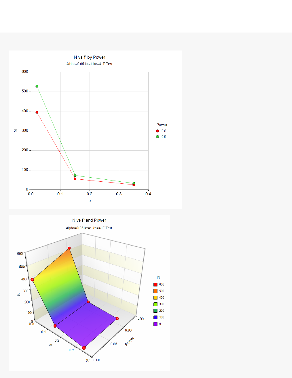
Example 1 – Finding Sample Size in the Conditional Model
Suppose researchers are planning a multiple regression study to look at the impact of a fifth independent
variable on the overall F test. They want to determine the sample size requirements needed to detect a
small, medium, or large effect. They want to consider power values of either 0.8 or 0.9 and a significance
level is 0.05. They know the X’s in advance, so they want to use the conditional model for power calculations.
Setup
If the procedure window is not already open, use the PASS Home window to open it. The parameters for this
example are listed below and are stored in the Example 1 settings file. To load these settings to the
procedure window, click Open Example Settings File in the Help Center or File menu.
Design Tab
_____________ _______________________________________
Solve For ....................................................... Sample Size
Power............................................................. 0.8 0.9
Alpha.............................................................. 0.05
Regression Model Type ................................. Conditional (Fixed X’s)
kc ................................................................... 4
kT ................................................................... 1
f 2 ................................................................... 0.02 0.15 0.35

PASS Sample Size Software NCSS.com
Multiple Regression using Effect Size
868-6
© NCSS, LLC. All Rights Reserved.
Output
Click the Calculate button to perform the calculations and generate the following output.
Numeric Reports
Numeric Results
─────────────────────────────────────────────────────────────────────────
Solve For: Sample Size
Model: Conditional (Fixed X's)
─────────────────────────────────────────────────────────────────────────
Number of
Independent Variables (X's)
Sample ──────────────────── Effect
Size Controlled Tested Size
Power N kc kт f² Alpha
─────────────────────────────────────────────────────────────────────────────────────────
0.8006 395 4 1 0.02 0.05
0.8039 55 4 1 0.15 0.05
0.8012 25 4 1 0.35 0.05
0.9004 528 4 1 0.02 0.05
0.9034 73 4 1 0.15 0.05
0.9058 33 4 1 0.35 0.05
─────────────────────────────────────────────────────────────────────────
Power The probability of rejecting a false null hypothesis when the alternative hypothesis is true.
N The number of observations on which the multiple regression is computed.
kc The number of independent variables controlled (i.e., those variables whose influence is removed from experimental
error).
kт The number of independent variables tested (i.e., those variables whose regression coefficients are tested against
zero).
f² Effect Size. Cohen interpreted Small = 0.02, Medium = 0.15, and Large = 0.35. f² = R²(T|C) / [1 - R²(C) - R²(T|C)],
where R²(C) is the R² value of only the control variables and R²(T|C) is the amount added to the overall R² value by
the treatment variables after the control variables.
Alpha The probability of rejecting a true null hypothesis.
Summary Statements
─────────────────────────────────────────────────────────────────────────
A multiple regression (Y versus X's) design, with 1 independent variable tested and 4 independent variables
controlled, will be used to test whether the R² of the test variable (above the R² of the control variables) is greater
than 0 (H0: R²(T|C) = 0 versus H1: R²(T|C) > 0). This corresponds to a test of whether the regression coefficient of
the test variable (given the control variables) is different from 0. The comparison will be made using a multiple
regression full-versus-reduced-model F-test, with a Type I error rate (α) of 0.05. The sample X values are assumed
to be fixed and known (the test is conditional upon known X values). To detect an effect size (f² = R²(T|C) / [1 -
R²(C) - R²(T|C)]) of 0.02 with 80% power, the number of needed subjects will be 395.
─────────────────────────────────────────────────────────────────────────

PASS Sample Size Software NCSS.com
Multiple Regression using Effect Size
868-7
© NCSS, LLC. All Rights Reserved.
Dropout-Inflated Sample Size
─────────────────────────────────────────────────────────────────────────
Dropout-
Inflated Expected
Enrollment Number of
Sample Size Sample Size Dropouts
Dropout Rate N N' D
─────────────────────────────────────────────────────────────────────────────
20% 395 494 99
20% 55 69 14
20% 25 32 7
20% 528 660 132
20% 73 92 19
20% 33 42 9
─────────────────────────────────────────────────────────────────────────
Dropout Rate The percentage of subjects (or items) that are expected to be lost at random during the course of the study
and for whom no response data will be collected (i.e., will be treated as "missing"). Abbreviated as DR.
N The evaluable sample size at which power is computed. If N subjects are evaluated out of the N' subjects that
are enrolled in the study, the design will achieve the stated power.
N' The total number of subjects that should be enrolled in the study in order to obtain N evaluable subjects,
based on the assumed dropout rate. After solving for N, N' is calculated by inflating N using the formula N' =
N / (1 - DR), with N' always rounded up. (See Julious, S.A. (2010) pages 52-53, or Chow, S.C., Shao, J.,
Wang, H., and Lokhnygina, Y. (2018) pages 32-33.)
D The expected number of dropouts. D = N' - N.
Dropout Summary Statements
─────────────────────────────────────────────────────────────────────────
Anticipating a 20% dropout rate, 494 subjects should be enrolled to obtain a final sample size of 395 subjects.
─────────────────────────────────────────────────────────────────────────
References
─────────────────────────────────────────────────────────────────────────
Cohen, Jacob. 1988. Statistical Power Analysis for the Behavioral Sciences, Lawrence Erlbaum Associates,
Hillsdale, New Jersey.
Gatsonis, C. and Sampson, A.R. 1989. 'Multiple Correlation: Exact Power and Sample Size Calculations.'
Psychological Bulletin, Vol. 106, No. 3, Pages 516-524.
─────────────────────────────────────────────────────────────────────────
This report shows the necessary sample sizes. The definitions of each of the columns is given in the Report
Definitions section.

PASS Sample Size Software NCSS.com
Multiple Regression using Effect Size
868-9
© NCSS, LLC. All Rights Reserved.
Example 2 – Validation
We will use an example from the Multiple Regression procedure to validate this procedure. Example 5 of that
procedure calculates a power of 0.9683 when alpha = 0.05, N = 15, k
T
= 2, and R
2
= 0.6. To use this procedure,
we must translate the R
2
value to an f
2
value. Using the relationship
=
|
1
|
we find
=
0.6
1 0.0 0.6
= 1.5
Setup
If the procedure window is not already open, use the PASS Home window to open it. The parameters for this
example are listed below and are stored in the Example 2 settings file. To load these settings to the
procedure window, click Open Example Settings File in the Help Center or File menu.
Design Tab
_____________ _______________________________________
Solve For ....................................................... Power
Alpha.............................................................. 0.05
N .................................................................... 15
Regression Model Type ................................. Conditional (Fixed X’s)
kc ................................................................... 0
k
T
................................................................... 2
f
2
.................................................................... 1.5
Output
Click the Calculate button to perform the calculations and generate the following output.
Numeric Results
─────────────────────────────────────────────────────────────────────────
Solve For: Power
Model: Conditional (Fixed X's)
─────────────────────────────────────────────────────────────────────────
Number of
Independent Variables (X's)
Sample ──────────────────── Effect
Size Controlled Tested Size
Power N kc kт f² Alpha
─────────────────────────────────────────────────────────────────────────────────────────
0.9683 15 0 2 1.5 0.05
─────────────────────────────────────────────────────────────────────────
The power of 0.9683 matches the result in the other procedure.
