
SM Journal of
Biometrics &
Biostatistics
Gr up
SM
How to cite this article Looney SW. Practical Issues in Sample Size Determination
for Correlation Coefcient Inference. SM J Biometrics Biostat. 2018; 3(1): 1027.
OPEN ACCESS
ISSN: 2573-5470
Introduction
An important issue in planning any study that will require inference for a correlation coecient
is the determination of the appropriate sample size to use. e usual procedure of choosing n based
on the power of the test of the hypothesis that the population correlation is zero oen results in
correlations of little practical importance being declared "signicant," and condence intervals that
are too wide to be of any practical use. In this article, alternative methods for determining sample
size are presented and compared to the "usual" procedure.
Example
Suppose that one is planning a study involving bivariate normal data in which statistical
inference is to be performed for a Pearson Correlation Coecient (PCC) and that the consensus of
previous research in the area is that the population correlation is no smaller than 0.40. Reference
to sample size tables for the "usual" t-test of the correlation coecient [1] indicates that a sample of
n= 46 will yield 80% power for detecting departures from zero as small as ρ = 0.40 when α = 0.05
(Table 1).
For the sake of argument, suppose that the value of the sample PCC (denoted here aer by r)
from a subsequent sample of 46 is exactly equal to 0.40. is yields a 2-tailed p-value of 0.006 and a
95% condence interval of (0.12, 0.62). Although these results indicate statistical signicance, their
practical signicance is unclear because the condence interval is too wide to draw any reasonable
conclusion about the true magnitude of ρ. For example, Hebel and McCarter [2] classify 0.0 ≤ |ρ |
≤ 0.2 as "negligible," 0.2 < | ρ | < 0.5 as "weak," 0.5 ≤ | ρ | ≤ 0.8 as "moderate," and 0.8 < | ρ | ≤ 1.0 as
"strong." us, using their classication scheme, all we can conclude from a condence interval of
(0.12, 0.62) is that ρ is somewhere between "negligible" and "moderate" (inclusive). If one prefers to
interpret correlation coecients in terms of eect size, Cohen [1] suggests that one classify | ρ | = 0.1
as a "small" eect size, | ρ | = 0.3 as "medium," and | ρ | = 0.5 as "large." Using this scheme, all that a
condence interval of (0.12, 0.62) tells us is that the eect size of | ρ | is somewhere between "small"
and "large" (inclusive).
One of the alternative approaches proposed in this article is to select n on the basis of the desired
width of the resulting Condence Interval (C.I.) for ρ rather than the power of the test of H
0
: ρ= 0.
For the aforementioned example, Table 2 indicates that a sample size of n = 273 is required to yield
a 95% C.I. of width 0.20 using a "planning value" of r = 0.40. Assuming that a value of exactly r =
0.40 is obtained from a subsequent sample of 273, the resulting p-value is <0.001 and the 95% C.I.
is (0.30, 0.50). While this result also indicates statistical signicance, the C.I. is suciently narrow
to indicate that the population correlation between the two variables is "weak" according to the
classication scheme of Hebel and McCarter.
Background
e diculty described in the previous section arises primarily from the fact that H
0
: ρ= 0 is
not the appropriate null hypothesis to test in most situations that require inference for a single
Research Article
Practical Issues in Sample Size
Determination for Correlation
Coecient Inference
Stephen W Looney*
Department of Population Health Sciences, Augusta University, USA
Article Information
Received date: Mar 12, 2018
Accepted date: Mar 19, 2018
Published date: Mar 22, 2018
*Corresponding author
Stephen W Looney, Department of
Population Health Sciences, Augusta
University, USA, Tel: (706) 721 4846;
Email: [email protected]
Distributed under Creative Commons
CC-BY 4.0
Keywords Condence Interval; Fisher
Z-Transform; Hypothesis Test; Interval
Width; Kendall Coefcient; Pearson
Correlation; Spearman Correlation;
Statistical Power
Abstract
Determination of the appropriate sample size to use when performing inference for a single Pearson
correlation coefcient ρ is usually based on achieving sufcient power for the test of H
0
: ρ = 0. However, sample
sizes found using this method can yield condence intervals that are so wide that they provide very little useful
information about the magnitude of the population correlation. Alternative approaches for determining the
appropriate sample size are proposed and compared to the "usual" method.
Citation: Looney SW. Practical Issues in Sample Size Determination for
Correlation Coefcient Inference. SM J Biometrics Biostat. 2018; 3(1): 1027.
Page 2/4
Gr up
SM
Copyright Looney SW
correlation coecient. It is usually of little interest to determine if
there is sucient evidence to conclude that ρ = 0. (An exception would
be a study in which the primary null hypothesis is that variables X and
Y are independent and X and Y can be assumed to have a bivariate
normal distribution.) Most investigators would not proceed with a
study unless they had sucient reason to believe that the population
correlation is non-zero, even though no formal statistical hypothesis
test had ever been performed. Other authors agree with our assertion:
Strike [4] argues that the test of ρ = 0 is "utterly redundant" and
Shoukri [5] asserts that a test of H
o
: ρ = 0 is "meaningless."
Another problem with testing H
o
: ρ = 0 is that the usual t-test
oen rejects the null hypothesis for small values of the sample
correlation, even when the sample size is small to moderate (Table
3). For example, when n = 30, a sample value of r = 0.361 ("weak,"
according to [2]) yields p = 0.05 (but note the extremely wide C.I. of
(0.001, 0.638)). For a sample of n = 100, a correlation of only 0.197
yields p = 0.05. is correlation is "negligible" according to [2] and
would be classied as a small eect size by Cohen [1]. Since the
width of a C.I. for ρ varies inversely with both the sample size and
the magnitude of r, the combination of small r and small to moderate
n oen yields C.I.'s that are too wide to be of any practical use, even
though p < 0.05.
A further concern is that the sample sizes required to yield 80%
or 90% power for testing H
o
: ρ = 0 are generally too small to yield
C.I.'s of a usable width, even when the sample correlation is large
(Table 1). For example, a sample of only n = 6 is required to achieve
80% power against the alternative value ρ
1
= 0.90. Assuming that the
value of r from a subsequent sample of n = 6 is exactly equal to 0.9
yields p = 0.015 and a 95% C.I. of (0.33, 0.99) (Table 1), which merely
indicates that ρ is somewhere between "weak" and "strong" (inclusive)
according to [2]. If Cohen's Classication based on eect size is used,
this interval only tells us that the eect size of ρ is at least "medium"
in magnitude [1].
Alternative Approaches
One alternative to testing H
o
: ρ = 0 is to specify another null value.
Sometimes one is interested primarily in determining if the sample
results are consistent with some relevant non-zero hypothesized
value; for example, the smallest value of the correlation that would
be considered to be clinically meaningful. Such a value may be
determined from examining previously published research in the
area, from published guidelines or recommendations, from the
clinical judgment and expertise of the research team, etc. Applying
the Fisher z-transform to r,
yields a new random variable that has an approximate normal
distribution with mean 0 and variance 1/(n - 3). is result can be
used to derive a test statistic for testing H
0
: ρ= ρ
0
:
(1)
Table 3: Condence intervals corresponding to minimum value of r required to
yield p ≤ 0.05 when testing H
0
: ρ= 0 (2-tailed test).
Sample Size Minimum r Yielding p ≤ 0.05 95% C.I.(ρ) Width of C.I./2
10 0.632 (0.004, 0.903) 0.45
20 0.444 (0.002, 0.741) 0.37
30 0.361 (0.001, 0.638) 0.319
40 0.312 (0.001, 0.568) 0.284
50 0.279 (0.001, 0.517) 0.259
60 0.255 (0.001, 0.478) 0.239
70 0.235 (0.000, 0.445) 0.223
80 0.22 (0.000, 0.419) 0.21
90 0.208 (0.001, 0.398) 0.199
100 0.197 (0.001, 0.379) 0.19
120 0.18 (0.001, 0.348) 0.174
150 0.161 (0.001, 0.313) 0.157
180 0.147 (0.001, 0.287) 0.144
200 0.139 (0.000, 0.272) 0.136
0
(
,
n 3
z r)- z( )
z
ρ
=
−
0
( )
1 1 r
log ,
2 1 r
z r
+
=
−
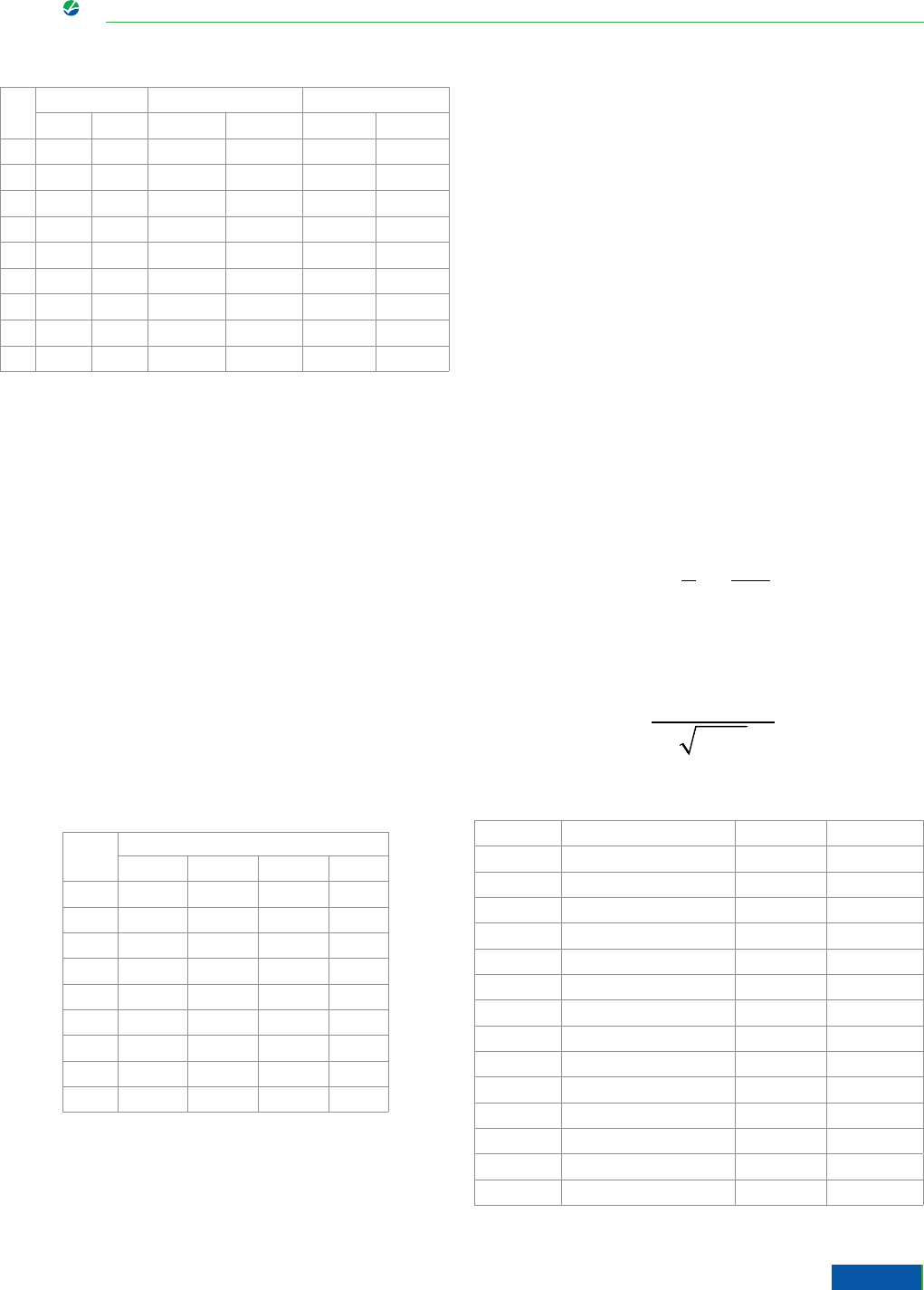
Table 1: Sample size required to achieve specied power (1 -β) for detecting ρ =
ρ1 when testing H
0
: ρ=0 using α = 0.05 (2-tailed test).
ρ1
Sample Size 95% CI if r=ρ1 2-tailed ρ-value if r=ρ1
β=0.10 β=0.20 β=0.10 β=0.20 β=0.10 β=0.20
0.1 1047 783 (0.04,0.16) (0.03,0.17) 0.001 0.005
0.2 259 194 (0.08,0.31) (0.06,0.33) 0.001 0.005
0.3 113 85 (0.12,0.46) (0.09,0.48) 0.001 0.005
0.4 62 46 (0.17,0.59) (0.12,0.62) 0.001 0.006
0.5 37 28 (0.21,0.71) (0.16,0.74) 0.002 0.007
0.6 24 18 (0.26,0.81) (0.18,0.83) 0.002 0.009
0.7 16 12 (0.31,0.89) (0.21,0.91) 0.003 0.011
0.8 11 9 (0.38,0.95) (0.29,0.96) 0.003 0.01
0.9 7 6 (0.46,0.99) (0.33,0.99) 0.006 0.015
The sample sizes in this table were obtained from Cohen [1].
Table 2: Minimum Sample Size Required to Yield a 95% C.I.(ρ) of Specied
Width
*
.
r
Width of 95% CI(r)
0.1 0.2 0.3 0.4
0.1 1507 378† 168† 95†
0.2 1417 355 159 90†
0.3 1274 320 143 81
0.4 1086 273 123 70
0.5 867 219 99 57
0.6 633 161 74 43
0.7 404 105 49 30
0.8 205 56 28 18
0.9 63 21 14 11
*e sample sizes in this table were obtained using the methods
of Bonett and Wright [3].
†Condence intervals based on these values of n and r are
guaranteed to contain ρ = 0, resulting in a failure to reject H
0
: ρ= 0.

Citation: Looney SW. Practical Issues in Sample Size Determination for
Correlation Coefcient Inference. SM J Biometrics Biostat. 2018; 3(1): 1027.
Page 3/4
Gr up
SM
Copyright Looney SW
where n is the sample size, z(r) is the Fisher z-transform applied
to the sample value of the PCC, and z (ρ
0
) is the Fisher z-transform
applied to the hypothesized value of the PCC, which can be any ρ
0
such that | ρ
0
| < 1. (Most commonly, ρ
0
= 0, in which case z (ρ
0
) =z
(0) =0.) e value of z
0
in (1) is then evaluated against the standard
normal distribution to obtain an approximate p-value.
In some instances, there may be no non-zero null value ρ
0
that is
of primary interest. In this case, one could use the cutos advocated
by Hebel and McCarter [2] (or other cutos that make sense in the
context of the applied problem) to get a sense of the magnitude of
the correlation in the population under study. For example, if it is
known that ρ is positive, then one could test H
0
: ρ≤ 0.8 to determine
if the population correlation is "strong" or H
0
: ρ ≤ 0.2 to determine
if the population correlation is "non-negligible" using the Hebel and
McCarter criteria. Tables similar to Table 1 could then be constructed
for these values of ρ
0
. Alternatively, using the same notation as in
Table 1, the following formula could be used for a 1-tailed test:
(2)
where z
r
denotes the upper
γ
-percentage point of the standard
normal and z(ρ) denotes the Fisher z-transform of ρ.
Consider the example discussed previously in which one wishes
to determine the appropriate sample size to use for a future study in
which the PCC is of primary interest and there is reason to believe
that ρ is positive and no smaller than 0.40. One approach would be
to test H
0
: ρ≤0.2; if this hypothesis is rejected, then one can conclude
that the population correlation is non-negligible according to [2]. A
calculation using Equation (2) indicates that samples of 130 and 179
would be required to achieve 80% and 90% power, respectively, to
detect ρ
1
= 0.40 using an upper-tailed test.
Suppose that a subsequent sample of n = 130 yielded a sample
value of exactly r = 0.40; the corresponding upper-tailed p-value for
the test of H
0
: ρ ≤ 0.2 is 0.006 and the one-sided 95% C.I. is (0.27, 1.00).
us, one can conclude that the population correlation is signicantly
greater than 0.2 (p < 0.001) and can be classied as "non-negligible”
according to [2]. In the example in which n = 30 and r = 0.361, the
p-value for the test of H
0
: ρ < 0.2 is 0.181, insucient evidence to
conclude that the population correlation is "non-negligible," despite
the fact that the test of H
0
: ρ=0 indicated that the result is “signicant.”
Another alternative is to focus one's attention on condence
interval estimation of the population correlation (derived using the
Fisher z-transform of r) instead of the test of a particular hypothesized
null value. is approach is consistent with the emphasis placed
on condence interval estimation over hypothesis testing by many
authors [6-8] Table 2 can be used to determine the sample size
required to obtain a 95% C.I. for ρ of a desired width. (is approach
was illustrated in a previous section).
Discussion
e purpose of this article is to illustrate some of the practical
problems encountered when attempting to determine the appropriate
sample size to use when a proposed study requires inference for a
single correlation coecient. e argument is made that H
0
: ρ= 0
is usually not the appropriate null hypothesis to test and that using
sample sizes that yield a desirable level of power (say, 80% or 90%)
for this test can result in C.I.'s that are so wide that they provide
very little useful information about the magnitude of the population
correlation. Two alternative approaches were proposed: (1) testing
null values other than ρ
0
= 0 and (2) determining the sample size so as
to achieve a certain level of precision of the estimate of ρ, as measured
by the width of the resulting C.I. Depending on the purpose of the
statistical analysis, either or both of these approaches could be a
useful alternative to the "usual" method of determining sample size.
However, it must be noted that the sample sizes required for either
of these approaches oen will be much larger than those required
to achieve acceptable power when testing H
0
: ρ= 0 . In the example
considered in a previous section, the “usual” approach based on
testing H
0
: ρ= 0 yielded a sample of size n = 46, the approach based
on testing H
0
: ρ ≤ 0.2 yielded n = 163 and the “C.I.” approach yielded
n = 273.
e alternative approaches described in this article could also be
applied if one were performing inference for the Spearman Correlation
Coecient (SCC) or the Kendall Coecient of Concordance (KCC).
For example, using the same notation as in Equation (2) for a one-
tailed test of the KCC, the "z-transform" developed by Fieller, Hartley,
and Pearson [9] for the KCC yields the sample size formula.
Where τb
0
and τb
1
are the null and alternative values of the KCC,
respectively (τb1 > τb0). For the SCC, the Fieller, Hartley and Pearson
z-transform yields.
(3)
where ρs
0
and ρs
1
are the null and alternative hypothesized values
of the SCC, respectively (ρs
1
>ρs
0
). Using the improved z-transform
of the SCC proposed by Bonett and Wright [3], the formula in (3)
becomes
(4)
Bonett and Wright recommend that (4) be used for | ρ
s1
| < 0.95
and that (3) be used if | ρ
s1
| ≥0.95.
We are not necessarily advocating the use of the Hebel and
McCarter criteria [2] for interpreting the magnitude of correlation
coecients. While we have found these to be useful in our own
exploratory analyses of biomedical data, they may not be appropriate
in other areas of investigation. However, we encourage the
development and use of such guidelines because we feel that they can
greatly enhance one's ability to interpret and communicate results
to non-statisticians (e.g., see the guidelines proposed by Landis and
Koch [10] for interpreting agreement coecients. And the guidelines
proposed by Fleiss et al. [11] for interpreting intra-class correlation
coecients).
( ) ( )
2
z z
4 0.437
z z
n
α β
+
= +
τ − τ
b1 b0
( ) ( )
2
s1 s0
z z
3 1.06 ,
z z
n
ρ ρ
α β
+
= +
−
( ) ( )
2
2
s1
s1 s0
z z
3 1 .
2 z z
n
ρ ρ
α β
+
ρ
= + +
−
2
1 0
3 ,
( ) ( )
z z
n
z z
α β
ρ ρ
+
= +
−

Citation: Looney SW. Practical Issues in Sample Size Determination for
Correlation Coefcient Inference. SM J Biometrics Biostat. 2018; 3(1): 1027.
Page 4/4
Gr up
SM
Copyright Looney SW
Simply reporting that a correlation is "signicant" just because
the p-value for the test of H
0
: ρ= 0 is less than 0.05 is generally not
sucient.
Acknowledgement
Some of this work was completed while the rst author was Acting
Senior Research Fellow in Epidemiology, Department of Medicines
Management and Visiting Professor, Department of Mathematics,
Keele University, Staordshire, England. is research was partially
supported by Wellcome Research Travel Grant #0816.
References
1. Cohen J. Statistical Power Analysis for the Behavioral Sciences. Hillsdale,
NJ: Lawrence Erlbaum Associates. 1988; 79-80,101.
2. Hebel JR, McCarter RJ. A Study Guide to Epidemiology and Biostatistics.
Burlington, MA: Jones and Bartlett Learning. 2012; 90.
3. Bonett DG, Wright TA. Sample size requirements for estimating Pearson,
Kendall, and Spearman correlations. Psychometrika. 2000; 65: 23-28.
4. Strike PW. Assay method comparison studies, in Measurement in Laboratory
Medicine: A Primer on Control and Interpretation, Oxford, UK: Butterworth-
Heinemann. 1996; 170.
5. Shoukri MM. Measures of Interobserver Agreement and Reliability. Boca
Raton, FL: CRC Press 2011; 92.
6. Gardner MJ, Altman DG. Condence intervals rather than P values:
Estimation rather than hypothesis testing. British Medical Journal 1986; 292:
746-750.
7. Hahn GJ, Meeker WQ. Statistical Intervals. New York: John Wiley & Sons.
1991; 39-40.
8. Schmidt F. Statistical signicance testing and cumulative knowledge in
psychology: Implications for training of researchers. Psychological Methods.
1996; 1: 115-119.
9. Fieller EC, Hartley HO, Pearson ES. Tests for rank correlation coefcients. I.
Biometrika 1957; 44: 470-481.
10. Landis JR, Koch GG. The measurement of observer agreement for categorical
data. Biometrics. 1975; 33: 159-174.
11. Fleiss JL, Levin B, Paik MC. Statistical Methods for Rates and Proportions,
Hoboken, NJ: John Wiley & Sons. 2003; 604.
