arXiv:2207.11332v2 [stat.AP] 24 Apr 2024

Comparing baseball players across eras via novel

Full House Modeling

Shen Yan

, Adrian Burgos Jr.

, Christopher Kinson

and Daniel J. Eck

1∗

April 25, 2024

1. Department of Statistics, University of Illinois Urbana-Champaign

2. Department of History, University of Illinois Urbana-Champaign

Abstract

A new methodological framework suitable for era-adjusting baseball statistics is devel-

oped in this article. Within this methodological framework speciﬁc models are motivated.

We call these models Full House Models. Full House Models work by balancing the achieve-

ments of Major League Baseball (MLB) players within a given season and the size of the

MLB talent pool from which a player came. We demonstrate the utility of Full House

Models in an application of comparing baseball players’ performance statistics across eras.

Our results reveal a new ranking of baseball’s greatest players which include several modern

players among the top all-time players. Modern players are elevated by Full House Model-

ing because they come from a larger talent pool. Sensitivity and multiverse analyses which

investigate the how results change with changes to modeling inputs including the estimate

of the talent pool are presented.

Keywords: Order statistics, Nonparametric estimation, Extrapolation techniques, Era-adjustment,

Sports statistics.

∗

email addresses: Shen Yan ([email protected]); Adrian Burgos Jr. ([email protected]); Christo-

pher Kinson ([email protected]); Daniel J. Eck ([email protected])

arXiv:2207.11332v2 [stat.AP] 24 Apr 2024

1 Introduction

Debating which baseball players are the best of all-time is a fun exercise among baseball fans.

There are many statistics for measuring the greatness of players, and these statistics are often

used as justiﬁcation in these debates. Career or peak oﬀensive or pitching statistics such as home

runs, batting average, runs batted in, earned run average, strikeouts and pitcher wins used to

dominate discussions of baseball players. Sabermetricians and Statisticians investigated more

nuanced measures of a player’s abilities, see [Thorn and Palmer, 1984, McCracken, 2001, Albert

and Bennett, 2003, Lewis, 2003, Tango et al., 2007, Bullpen, 2023]. These investigations led to

the creation of on-base plus slugging percentage, weighted on-base average, ﬁeld independent

pitching. Various adjustments to these statistics to account for stadium eﬀects, league eﬀects,

and batted ball proﬁle of a batter or batted ball proﬁle allowed of a pitcher have led to even better

measures of a player’s ability. One statistic in particular that has captured the imagination of

baseball fans is wins above replacement, abbreviated as WAR [Baumer and Matthews, 2014,

Bullpen, 2023]. WAR is an attempt by the sabermetric baseball community to summarize a

player’s total contributions to their team in one statistic [Slowinski, 2010]. There are several

proprietary versions of WAR that exist with Baseball Reference WAR, often denoted bWAR

or rWAR [Forman, 2010], and Fangraph’s WAR, denoted fWAR [Slowinski, 2010], and WARP

[Baseball Prospectus Staﬀ, 2013] being the most popular. In addition to these versions of WAR,

there exists openWAR that is based on public data and careful transparent methodology [Baumer

et al., 2015]. There is no shortage of statistics for individuals to quote when they passionately

argue for who they think are the greatest baseball players ever.

Debates about the all-time greatest baseball players often involve comparisons of players who

accrued their statistics in vastly diﬀerent eras. This makes for lively debate as people present their

cases for or against the relative merit of statistics from diﬀerent time periods. There are many

factors that contribute to the diﬀerences of eras that are separated in time. Some factors include

population size, Westward and Southern expansion of the USA and baseball, league expansion

and team relocation, changing interest levels in baseball, erosion of the Minor Leagues, changing

approaches to playing baseball, changing managerial strategies, integration, globalization, wars,

international relations, changing salaries, changing modes of transportation, changing training

methods, medical technology, changing media environments, etc. [Land et al., 1994, Gould, 1996,

Schmidt and Berri, 2005, Burgos Jr, 2007, Rader, 2008, Armour and Levitt, 2016, Eck, 2020a,b].

A starting place for confronting the vast era diﬀerences can be found in the work of Stephen

Jay Gould. Gould [1996] suggested that the entire distribution of achievement, or “full house of

variation,” is relevant when considering the achievements of baseball players across eras. This

idea was also recognized as the starting place for an answer by Schell [1999] and Schell [2005].

These works consider seasonal standard deviations as a proxy for changing eras. Berry et al.

[1999] assumed that the changing talent pool is captured by seasonal random eﬀects. Berry et al.

[1999] also considered overlapping player aging curves as a way to establish bridges across eras.

In addition to all of the sophisticated statistics approaches, there are several websites and books

which provide their own lists of the greatest baseball players using a combination of statistics and

opinion [ESPN, 2022], variations of WAR [of Stats, 2022], and painstaking narrative curation

informed by a plethora of statistics and context considerations [Posnanski, 2021].

Our contribution to these discussions is a novel modeling approach that extends Gould’s

“full house of variation” concept to the talent pool. This method works by using an estimate

of the size of the talent pool as a modeling input and connecting order statistics of observed

MLB statistics to individuals in the talent pool. With distributional assumptions placed on the

process that assigns latent talent to individuals in the talent pool, an assumption that the most

talented people are in the MLB, and a pairing between observed statistics and latent talent

such that the best performer according to a particular metric is paired with the highest latent

talent, the second best performer is paired with the second most talented individual and so on,

we can estimate the latent talent values of MLB players. These mechanics allow for a balancing

between how far one stands from their peers and the size of the talent pool. To have a high talent

score, one must stand out from their peers in their own time and be a product of a large talent

pool. Historically great players like Babe Ruth, Ty Cobb, Lefty Grove, and Walter Johnson, to

name a few, dwarfed their contemporaries by such a degree that they remain among the all-time

greatest players despite playing in eras that we estimate to have small talent pools relative to

more modern eras.

We argue that our results indicate an era-neutral ranking of baseball players. However, it

is very important to note that this claim is built on the assumption that we have properly

estimated the talent pool. Our estimation of the talent pool is discussed in this article and in

our Supplementary Materials. Our rankings reveal that more modern baseball players now sit

atop the lists of baseball’s greatest than many other approaches. For example, our era-adjusted

versions of bWAR (ebWAR) and fWAR (efWAR) favor Barry Bonds and Willie Mays over Babe

Ruth. A detailed investigation into how we estimated the talent pool for each season will be

provided. Sensitivity analyses, multiverse analyses [Steegen et al., 2016], and alternate talent

pool estimates will be considered. We now present Full House Modeling through an application

of comparing baseball players across eras.

2 Full House Model Setting

Let N

denote the size of the talent pool in year i. We will suppose that every individual

j = 1, . . . , N

has an underlying talent value X

i,j

iid

∼ F

. We denote X

i,(j)

as the jth ordered

talents in year i. We deﬁne g

(·, ·) as the MLB inclusion function, where g

i,j

, X

i,−j

) = 1

indicates that individual j is an active MLB player in the ith year, and g

i,j

, X

i,−j

) = 0

indicates that individual j is not an active MLB player in the ith year. Let X

i,−j

be the vector

of all individual talents not including the component j. We will assume that the most talented

individuals from the talent pool in year i are active players in the MLB so that

i,j

, X

i,−j

) = 1



i,j

≥ X

i,(N

−n

+1)



, (1)

where n

is the number of active MLB players in year i and 1(·) is the indicator function. Note

that: 1) our estimation of the talent pool accounts for changing interest in baseball over time;

2) it is likely that there are potential players not in the MLB that have more talent in a certain

area than some active MLB players. That being said, we think it is sensible to assume that

those players would not be among the most talented players in the MLB if they were to be in

the MLB.

We now suppose that in year i an active MLB player j has an observed statistic Y

i,j

. For

example, Y

i,j

can be batting average or wins above replacement (WAR) per game. We suppose

that Y

i,j

iid

∼ F

where F

will be continuous. We denote Y

i,(j)

as the jth ordered statistic for

players in the MLB during year i. The key to the Full House Model is connecting talent values

X with observed statistics Y . This is achieved by assuming that outcome data Y arrives from

a pairing with X, (Y

i,(j)

, X

i,(N

−n

+j))

), j = 1, . . . , n

. As an example, the highest performer in

the MLB in year i as judged by values Y

i,j

will be assumed to have the highest talent score in

year i. More detail on this pairing is given in Sections 2.1 and 2.2.

2.1 Parametric distributions for baseball statistics

We now demonstrate how the Full House Model works in a parametric setting. Consider the

pair (Y

i,(j)

, X

i,(N

−n

+j)

) and suppose that the distribution corresponding to Y

i,j

from the ith

system is known to belong to a continuous parametric family indexed by unknown parameter θ

and let F

(· | θ

) be a parametric CDF with parameter θ

∈ R

. We can estimate θ

with

and plug the estimator into the CDF F

(· |

In order to connect the Y

i,(j)

and X

i,(N

−n

+j)

and obtain an estimate of the underlying

talents, we will make use of the following classical order statistics properties,



i,(j)

| θ



∼ U

i,(j)

, F



i,(j)



≈ U

i,(j)



i,(j)

| θ



∼ U

i,j

, F

i,(j)



i,(j)



≈ U

i,j

where ≈ means approximately distributed, ∼ means distributed as, U

i,j

∼ U(0, 1), and U

i,(j)

∼

Beta(j, n

+ 1 −j) and the quality of the approximation in the right-hand side depends upon the

estimator

and the sample size.

We now connect the order statistics to the underlying talent distribution that comes from a

population with N

≥ n

observations when F

is known. This connection is established with

−1

i,(N

−n

+j)



i,(j)



i,(j)

| θ



∼ F

−1

i,(N

−n

+j)



i,(j)



i,(j)



= X

i,(N

−n

+j)

. This is

estimated with

−1

i,(N

−n

+j)



i,(j)



i,(j)



≈ F

−1

i,(N

−n

+j)



i,(j)



i,(j)



= X

i,(N

−n

+j)

. (2)

2.2 Nonparametric distribution for baseball statistics

2.2.1 Past methods and challenges of nonparametric approach

The empirical cumulative distribution function (CDF)

is a widely used nonparametric ap-

proach in estimating the CDF. However,

fails in our setting because

i,(n

)

) = 1 which,

when mapped to X values through a similar approach to (2), yields X

i,(N

)

= sup

{x : F

(x) <

1}. The implication here is that the highest achiever in year i is estimated to have maximal pos-

sible talent, and this is nonsense. Therefore, we have an extrapolation problem. There are many

alternatives to

. For example, one could use piecewise linear function estimation [Leenaerts

and Bokhoven, 1998, Kaczynski et al., 2012], kernel estimation [Silverman, 1986], and semi-

parametric conjugated estimation [Scholz, 1995]. One could also consider parametric families of

the generalized Pareto distribution that have ﬂexible behavior in both tails [Stein, 2020].

All methods above, and others not mentioned, ﬁt within a more general Full House Modeling

paradigm than what we motivate here. However, in the application to baseball data, the range of

the distribution is naturally constrained, and outlying achievements are lauded for their rarity.

In preliminary analyses we found that several of the above methods led to era-adjusted results

that rewarded performances of top achievers that did not stand far above their peers. The main

issue for these methods was that a tight grouping of top achievers would result in the very highest

achiever having an extremely large estimated talent score when that player only stood a relatively

short distance higher than the other top achievers. We found that an approach motivated from

Scholz [1995] performed well with these issues. Details will be discussed in Section 2.2.3.

2.2.2 Handling extrapolation

In the nonparametric setting, we motivate a variant of a natural interpolated empirical CDF as

an estimator of the system components distribution F

to solve the problems mentioned in the

previous section. We consider surrogate sample points to construct an interpolated version of

the empirical CDF

and this type of interpolated CDF is a standard technique to replace the

empirical CDF [Kaczynski et al., 2012].

We construct the interpolated CDF in the following manner: We ﬁrst construct surrogate

sample points

i,(1)

= Y

i,(1)

− Y

∗

i,(j)



i,(j)

+ Y

i,(j−1)



/2, j = 2, . . . , n, and

i,(n

+1)

i,(n

)

+ Y

∗∗

, where Y

∗

is the value to construct the lower bound and Y

∗∗

is the value to

construct the upper bound. With this construction, we build

(t) =

j=1





j −1

t −

i,(j)



i,(j+1)

−

i,(j)









i,(j)

≤ t <

i,(j+1)



+ 1



t ≥

i,(n

+1)



(3)

The estimator

is desirable for three reasons. First, we found (3) to be quick computation-

ally. Second, we do not assume that the observed minimum and observed maximum constitute

the actual boundaries of the support of Y . Third,



i,(1)



and



i,(n

)



provide reasonable

estimates for the cumulative probability at Y

i,(1)

and Y

i,(n

)

by considering their respective value

of Y

∗

and Y

∗∗

. Here Y

∗∗

is chosen to measure how far the highest achiever in year i stood from

their peers where small values of Y

∗∗

−Y

i,(n

)

have the interpretation that Y

i,(n

)

is an outlying

performance and large values of Y

∗∗

− Y

i,(n

)

indicate the opposite.

The approximations to facilitate our methodology are similar to the ones in the paramet-

ric case. Latent talent values can be found as follows, F

−1

i,(N

−n

+j)



i,(j)



i,(j)



∼

−1

i,(N

−n

+j)



i,(j)



i,(j)



= X

i,(N

−n

+j)

. This can be estimated as

−1

i,(N

−n

+j)



i,(j)





i,(j)





≈ F

−1

i,(N

−n

+j)



i,(j)



i,(j)



= X

i,(N

−n

+j)

. (4)

Notice that

(t) was explicitly constructed to be close to

(t). We formalize this statement

in the Supplementary Materials.

2.2.3 Choosing Y

∗

and Y

∗∗

The cumulative probabilities



i,(1)



and



i,(n

)



are, respectively, functions of Y

∗

and

∗∗

. In this section, we describe the role of Y

∗

and Y

∗∗

and how these quantities are chosen

in our application to historical baseball rankings. The lower bound Y

∗

determines the lower

tail behavior of talent distribution, and in fact, most normal or low talents would concentrate

in a similar scale or size [Newman, 2005]. Therefore Y

∗

can be a small positive value, we deﬁne

∗

= Y

i,(2)

− Y

i,(1)

. This is not the only choice of Y

∗

, and other reasonable choices can also be

set to the Y

∗

We now discuss how we calculate Y

∗∗

. Our approach follows a simple nonparametric tail

extrapolation method motivated in Scholz [1995]. First, some preliminaries. The p-quantile y

of F is deﬁned as the smallest value for which F (y

) = p, i.e. y

= inf{y : F (y) ≥ p}. Hence

P (Y

i,j

≤ y

) = p. Now suppose that p

i,j,γ,n

is the value of p that satisﬁes γ = P



i,(j)

≥ y



For each j and γ there is an approximation of p

i,j,γ,n

for choices of γ [Scholz, 1995]. Hoaglin

et al. [1983] gave a speciﬁc justiﬁed approximation of p

i,j,γ,n

when γ = 0.5. This approximation

is,

i,j,.5,n

≈

j −

With this approximation, we have a tractable means to connect the order statistics Y

i,(j)

percentile values p

i,j,.5,n

corresponding to the median value of a quantile y

i,j,.5,n

Following Scholz [1995], we consider the regression ﬁt on points (h(p

i,j,.5,n

), Y

i,(j)

), j =

−k + 1, . . . , n

, where k is the number of extreme data values to use in the extrapolation step,

and h is a function of tail probabilities. The speciﬁc choices that we considered for h to model

tail probabilities are similar to those in Section 2 of Scholz [1995]:

• linear transformation: h

(p) = θ

+ θ

• logit transformation: h

(p) = θ

+ θ

log(p/(1 − p));

In practice, we chose h among the candidates by selecting whichever h maximized regression ﬁt

as judged by R

values.

The value of k is determined by a similar procedure to that in Section 5 of Scholz [1995]:

we specify that k ∈ [K

, K

] where K

= max(6, ⌊1.3

√

n⌋) and K

= 2 ⌊log

(n)

√

n⌋. We

then choose k as the value that maximizes adjusted R

values among regressions motivated in

Sections 3-4 of Scholz [1995]. We found that the regression approach in Section 3-4 of Scholz

[1995] suﬀered similar problems as those mentioned in the the last paragraph of Section 2.2.1.

With k and h selected, we then compute Y

∗∗

through a connection between

i,(n

)

) and

the regression ﬁt on points (h(p

i,j,.5,n

), Y

i,(j)

), j = n

− k + 1, . . . , n

. Speciﬁcally, we ﬁnd Y

∗∗

as the solution of the following optimization problem

∗∗

= argmin



−1

i,(n

)

) −

i,(n

)

; y)



, (5)

where

(·; y) is

deﬁned with respect to a value y replacing Y

∗∗

in its construction. The in-

tuition of (5) for large outlying values of Y

i,(n

)

is as follows: the value of h

−1

i,(n

)

) corresponds

to percentile p

i,n

,.5,n

that is close to 1, and this pulls Y

∗∗

towards zero so that

i,(n

)

) is

also close to 1.

2.3 Estimate how players will perform in a diﬀerent year

We can now reverse engineer the process above to obtain era-adjusted statistics in any context

that is desired. Consider the the pair (Y

i,(j)

, X

i,(N

−n

+j)

) in the ith year. We ﬁrst put the

talent value X

i,(N

−n

+1)

obtained by (2) or (4) in the new talent pool of desired year m and

reverse the process to obtain the hypothetical baseball statistics in year m, which we will denote

as Y

i,j,m

. The distribution F

is known.

More formally, Y

i,j,m

are computed as follows when baseball statistics are estimated para-

metrically:

i,j,m

= F

−1



−1

m,(l

i,j,m

)



m,(N

−n

i,j,m

))



i,(N

−n

+j)





, (6)

where l

i,j,m

is the rank of X

i,(N

−n

+j)

among the values



i,(N

−n

+j)

, X

m,(N

−n

+t))

: t = 1, . . . , n



. The baseball statistics Y

i,j,m

are computed as

follows when baseball statistics are estimated nonparametrically:

i,j,m

−1



−1

m,(l

i,j,m

)



m,(N

−n

i,j,m

)



i,(N

−n

+j)





. (7)

2.4 Putting it all together

We conclude Section 2 by expressing the working mechanics of the Full House Model in an

algorithmic format. Steps 1-3 describe how one obtains talents X from observations Y . Steps

4-6 describe how one reverse-engineers the process to obtain new Y values in a new context from

the talents in X computed in step 3. This algorithm is presented below:

Step 1: Input the statistics Y

i,1

, Y

i,2

, . . . , Y

i,n

, the talent pool size N

, and the number of active

MLB players n

for year i. Declare latent distribution X ∼ F

and system inclusion

mechanism g (1).

Step 2: Sort the components yielding Y

i,(1)

, Y

i,(2)

, . . . , Y

i,(n

)

Step 3. Obtain talent scores parametrically (2) or nonparametrically (4).

Step 4. Declare a setting for which hypothetical statistics Y

i,j,m

are desired.

Step 5. Apply steps 1-3 to extract talent scores for active MLB players in year m, {X

m,(N

−n

+t))

t = 1, . . . , n

}, and ﬁnd the rank l

i,j,m

of X

i,(N

−n

+j)

among these talent scores.

Step 6. Obtain statistics Y

i,j,m

parametrically (6) or nonparametrically (7).

The steps of the above algorithm are presented in Figure 1. This ﬁgure depicts the process

of obtaining era and park-factor-adjusted batting average (BA) for two league-leading players,

Ty Cobb and Tony Gwynn. We can see even though Ty Cobb’s BA in 1911 is larger than Tony

Gwynn’s BA in 1997, Tony Gwynn’s BA talent score is higher. In our Supplementary Materials

we conducted a multiverse analysis [Steegen et al., 2016] which compared Ty Cobb’s BA in 1911

and Tony Gwynn’s 1997 BA under multiple conﬁgurations of our modeling assumptions and data

pre-processing regimes. In this analysis, it was found that the vast majority of conﬁgurations

favored Tony Gwynn over Ty Cobb, and conﬁgurations that led to the opposite conclusion

involved modeling assumptions that are not satisﬁed.

3 Modeling assumptions and data considerations

3.1 Historical talent pool

An estimate of the talent pool is a central input needed for our model, and our results follow

from it. Here we detail the general approach that we employed to estimate the talent pool. Full

details can be found here:

https://htmlpreview.github.io/?https://github.com/ecklab/

era-adjustment-app-supplement/blob/main/writeups/MLBeligiblepop.html

Our estimate of the talent pool will be pegged to the population of aged 20-29 males from

the North East (NE) and Midwest (MW) region of the United States of America. Simply stated,

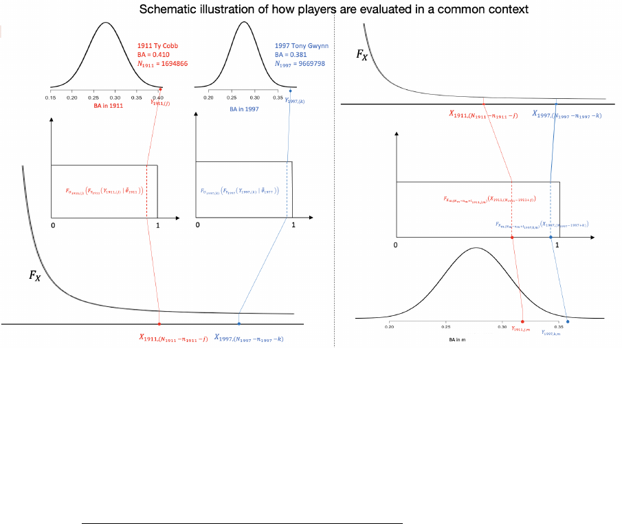
Figure 1: Obtaining era and park-factor adjusted batting averages for two players in diﬀerent seasons via the Full House

Model. The left panel illustrates how to extract the BA talent scores for Ty Cobb in 1911 and Tony Gwynn in 1997

using steps 1-3 in the Algorithm in Section 2.4. The right panel shows how to compute the era and park-factor adjusted

BA in a hypothetical season m for these players using steps 4-6 in the Algorithm in Section 2.4. Park-factor-adjusted

batting averages are assumed to be normally distributed.

the talent pool will be

NE and MW region population of age 20-29 males

proportion of MLB players from NE and MW regions

× adjustment.

Baseball started in the NE and MW regions. Our estimation approach tracks the talent pool as

baseball expands throughout the USA and abroad. We adjust for the eﬀects of changing interest

in baseball, wars, segregation, and gradual integration of the MLB.

The proportion of MLB players from the NE and MW regions can be calculated from using

birthplace information from the Lahman R package [Friendly et al., 2023]. We estimate the

talent pool from the NE and MW regions using US Census data and linear interpolation for

years in which we could not ﬁnd data. We have adjusted population sizes to account for the

eﬀects of wars, the rates of integration in the two traditional leagues which comprise the MLB

[Armour, 2007], and the changing interest in baseball as measured by Gallup and Harris (links

to speciﬁc polls are provided in the link at the beginning of this section). Baseball interest is

lagged by 10 years to reﬂect the level of baseball interest that was present when those in the

MLB were coming of age.

We deﬁne baseball interest to be the average of the proportion of people who are generally

interested in baseball and the proportion of people who list baseball as their favorite sport.

Including general interest in baseball is sensible because not everyone who plays baseball lists

baseball as their favorite sport, for example, Tony Gwynn loved basketball before baseball

. Av-

eraging these two sources of baseball interest yields an estimate of the talent pool that aligns with

a similarly constructed talent pool formed from select Latin American countries that are smaller

than the US in population but are more interested in baseball. Figures 2 and 3, respectively,

display our estimate of the talent pool and baseball interests over time.

Figure 4 shows that our estimate of the talent pool aligns with a similar talent pool computed

from the combination of the Dominican Republic, Puerto Rico, and Venezuela which are the

three countries with the most historical MLB players after the United States. This alignment

occurs from around 2005 to the present. Around 2005, a large inﬂux of Latin American players

began to level oﬀ [Armour and Levitt, 2016]. Separately, the Dominican Republic and Puerto

Rico exhibit over-representation in the MLB while Venezuela exhibits under-representation (see

Figure 4). Both of these ﬁndings are pronounced but are hardly surprising considering the

extensive development of baseball academies in the Dominican Republic and Puerto Rico, and

the recent relations between the USA and Venezuela.

3.2 Modeling assumptions and speciﬁcations

In Section 2 we supposed that the all N

individuals in population i have talents X

i,1

, . . . , X

i,N

iid

∼

. Here N

corresponds to the size of the talent pool in year i. The Full House Model results

displayed throughout Section 4 assumed that F

corresponds to a Pareto(α) distribution with

α = 1.16. This choice of α reﬂects the Pareto principle or “80-20 rule” [Pareto, 1964]. Berri

and Schmidt [2010] noted that the superstars are really important for their teams to win and

stated that about 80% of wins appear to be produced by the top 20% of players. Thus there

is some precedent for our assumption on F

. In the Supplementary Materials, we perform a

sensitivity analysis on choices of F

. This sensitivity analysis reveals that our conclusions do not

depend on the distribution assumed for F

, as expected since the ranking of players is preserved.

https://www.mlb.com/news/tony-gwynn-drafted-in-baseball-basketball-on-same-day

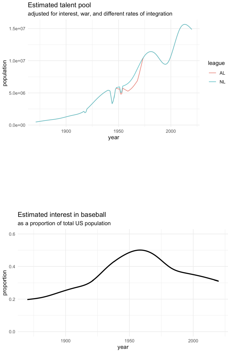
Figure 2: Estimated baseball talent pool over time.

Figure 3: Estimated interest in baseball over time.

Figure 4: MLB representation vs talent pool size for select Latin American countries. The countries considered are the

Dominican Republic (DR), Puerto Rico (PR), and Venezuela (Ven), and the combination of these three countries. The

blue line (MLB representation) is our estimated talent pool multiplied by the proportion of MLB players from these

Latin American countries. The red line (eligible pop) is the estimated talent pool for these Latin American countries.

All baseball statistics will be analyzed using our nonparametric method articulated throughout

Section 2.2. Handedness-speciﬁc park-factor adjustments are made to batting averages and home

run rates. These adjustments are computed using the same methods in Schell [2005].

The Full House Model results displayed throughout Section 4 were estimated in a common

context. Namely, we built a common mapping environment to evaluate all player seasons. Schell

[2005] inspired us to use the National League (NL) seasons from 1977 through 1989, excluding

the 1981 strike-shortened season, as the seasons comprising the common mapping environment.

Schell [2005] noted that the 1977-1989 NL represents possibly the most steady time in baseball

history for all of the fundamental oﬀensive occurrences. Additionally, no expansion occurred

over these years. We ﬁt an isotonic regression model with observed performance statistics on

estimated talent scores obtained from our Full House Model for all 1977-1989 NL player seasons,

excluding the 1981 strike-shortened season. We obtained predicted performance statistics (which

we will denote as

Y ) from this isotonic regression model to pair with estimated talent scores.

We set the number of players in the common mapping environment to be equal to the

maximum number of full-time players (denoted n) throughout the 1871-2023 seasons. Then

we select as data pairs to form the common mapping environment as (

(k)

, X

(k)

), k = 1, . . . , n

corresponds to the

th quantile of all (

Y , X) data pairs that formed the common mapping

environment. From here, steps 1-3 of the algorithm in Section 2.4 were applied to all MLB

player seasons individually, and steps 4-6 of the algorithm in Section 2.4 found era-adjusted

statistics within the context of the common mapping environment.

Further details about pre-processing and adjustments to batting statistics and pitching statis-

tics can be found in the Supplementary Materials.

4 Results

We present our era-adjusted rankings of baseball players. Tables 1 and 2 display the top 25 career

era-adjusted rankings for, respectively, batters and pitchers across several key statistics. Table 3

displays top-25 combined era-adjusted WAR and JAWS lists for batters and pitchers. JAWS is

the average of a players’ career WAR and the players’ total WAR from his seven best seasons.

Note that Babe Ruth’s WAR and JAWS combine his batting and pitching contributions. Table 4

displays top-25 era-adjusted four-year peak batting averages and at-bats per home run rates.

Our rankings favor more modern players who come from a larger talent pool than legendary

players of the past. We ﬁnd that Barry Bonds and Willie Mays move to the top of WAR-based

rankings lists for batters, and Roger Clemens, Greg Maddux, and Randy Johnson move to the

top of WAR-based ranking lists for pitchers. Interestingly, Lefty Grove, who dominated during

an era that was favorable to batters, jumps a few spots on WAR-based ranking lists. Moreover,

Lefty Grove paces those above him on a rate-basis (ebWAR or efWAR per innings pitched).

Several active players at the time of this writing populate our era-adjusted top-25 ranking lists.

And the legendary players of the past do not disappear. For example, Babe Ruth is the career

leader in home runs, has the third highest at bats per home run four-year peak, and is fourth in

career ebWAR, efWAR, ebJAWS, and efJAWS among all players.

Our career and peak era-adjusted home run ranking lists reward modern players because

they are products of a larger relative talent pool than past players, but it penalizes players from

the steroids era because players’ accomplishments are judged relative to their peers. Our career

and peak era-adjusted batting ranking lists reward top players from the era of the pitcher (1962-

1968) who achieved relatively pedestrian batting averages and home runs due to conditions that

favored pitchers such as expanded strike zones and high pitching mounds. Our peak batting

average ranking rewards present-day players (at the time of this writing) who stand far from

their peers at a time in which batting averages are much lower than in past eras (for example,

Luis Arreaz’s 2023 BA of 0.354 is the only season in which a qualiﬁed batter eclipsed 0.350 BA

since Josh Hamilton had a 0.359 BA in 2010). In our Supplementary Materials we report top-25

career and four-year peak batting average ranking list resulting from the assumption that batting

averages for full-time players follows a normal distribution. These lists are broadly similar to

what is seen in Table 4 with notable elevation to older era-players and declines to present-day

players (at the time of this writing). Also included in our Supplementary Materials is an analysis

which demonstrates that a normal distribution assumption placed on batting averages for full-

time players does not hold up to Shapiro-Wilk testing [Shapiro and Wilk, 1965] with the tests

overly rejecting nominal tolerance. For these reasons we have reported batting average results

that arise when no distribution is speciﬁed for batting averages.

Figure 5 displays estimates of the WAR that a hypothetical 2-WAR player in 2023 would

name ebWAR name efWAR name HR name BA

1 Barry Bonds 153.89 Barry Bonds 145.24 Babe Ruth 702 Tony Gwynn 0.342

2 Willie Mays 144.08 Willie Mays 135.39 Henry Aaron 689 Rod Carew 0.329

3 Henry Aaron 135.60 Henry Aaron 128.05 Albert Pujols 662 Ichiro Suzuki 0.327

4 Babe Ruth 127.29 Babe Ruth 120.44 Barry Bonds 654 Jose Altuve 0.327

5 Alex Rodriguez 120.29 Stan Musial 113.03 Reggie Jackson 578 Ty Cobb 0.320

6 Stan Musial 119.51 Alex Rodriguez 110.30 Willie Mays 577 Roberto Clemente 0.320

7 Ty Cobb 114.48 Ty Cobb 108.77 Mike Schmidt 561 Miguel Cabrera 0.320

8 Albert Pujols 111.86 Ted Williams 107.75 Alex Rodriguez 547 Joe DiMaggio 0.318

9 Mike Schmidt 109.58 Mike Schmidt 106.41 Frank Robinson 535 Wade Boggs 0.316

10 Rickey Henderson 109.08 Rickey Henderson 103.90 Ken Griﬀey Jr 528 Buster Posey 0.316

11 Ted Williams 107.86 Albert Pujols 97.34 Willie Stargell 528 Mike Trout 0.315

12 Tris Speaker 102.26 Joe Morgan 96.07 David Ortiz 521 Ted Williams 0.314

13 Joe Morgan 100.17 Frank Robinson 95.92 Willie McCovey 515 Freddie Freeman 0.314

14 Frank Robinson 99.93 Mel Ott 95.72 Harmon Killebrew 508 Joe Mauer 0.314

15 Mel Ott 99.74 Tris Speaker 95.13 Ted Williams 503 Stan Musial 0.313

16 Cal Ripken Jr 97.39 Rogers Hornsby 94.42 Mickey Mantle 502 Willie Mays 0.312

17 Rogers Hornsby 97.01 Mickey Mantle 94.30 Eddie Mathews 502 Bill Terry 0.312

18 Lou Gehrig 95.87 Cal Ripken Jr 93.24 Eddie Murray 498 Robinson Cano 0.311

19 Mickey Mantle 95.37 Lou Gehrig 92.98 Jimmie Foxx 493 Henry Aaron 0.310

20 Carl Yastrzemski 95.20 Carl Yastrzemski 92.64 Stan Musial 492 Derek Jeter 0.310

21 Adrian Beltre 95.01 Honus Wagner 89.81 Dave Winﬁeld 491 Vladimir Guerrero 0.310

22 Wade Boggs 92.51 Wade Boggs 87.91 Mark McGwire 489 Al Oliver 0.310

23 Roberto Clemente 91.37 Mike Trout 87.87 Jim Thome 484 Matty Alou 0.310

24 Eddie Collins 90.94 Eddie Mathews 86.38 Miguel Cabrera 480 Lou Gehrig 0.309

25 Mike Trout 90.43 Adrian Beltre 86.34 Lou Gehrig 479 Edgar Martinez 0.309

Table 1: Top 25 batting careers according to era-adjusted bWAR (ebWAR), era-adjusted fWAR (efWAR), era-adjusted

home runs, and era-adjusted batting average (minimum 5000 adjusted at-bats).

produce in other seasons. Interestingly, this plot does not perfectly mirror the talent pool

presented in Figure 2. In particular, a 2-WAR player in 2023 is estimated to barely exceed 2

WAR in the 1950s despite the talent pool being far larger in 2023. One reason for this is MLB

expansion. There were, respectively, 16 and 30 teams in the 1950s and 2023

. Fewer players

were separating a 2-WAR player from the maximum achiever in the 1950s than in 2023. Thus a

2-WAR player in the 1950s would correspond to a higher quantile of the ordered sample of latent

baseball talents than a 2-WAR player in 2023. This partially oﬀsets the fact that the talent pool

was larger in 2023 than it was in the 1950s.

4.1 A closer look at Barry Bonds and Babe Ruth peak home run

seasons

Table 4 shows that Barry Bonds and Babe Ruth, respectively, rank ﬁrst and third in four-year

peak home run rate. We unpack how our modeling works for the top three seasons by home run

https://en.wikipedia.org/wiki/Timeline_of_Major_League_Baseball

name ebWAR name efWAR name ERA name K

1 Roger Clemens 145.88 Roger Clemens 141.25 Clayton Kershaw 2.43 Nolan Ryan 6026

2 Greg Maddux 113.66 Greg Maddux 120.73 Pedro Martinez 2.61 Randy Johnson 5136

3 Randy Johnson 110.81 Randy Johnson 109.77 Greg Maddux 2.77 Roger Clemens 4752

4 Tom Seaver 104.31 Nolan Ryan 108.30 Lefty Grove 2.78 Steve Carlton 4221

5 Lefty Grove 102.54 Bert Blyleven 101.82 Roger Clemens 2.81 Walter Johnson 3888

6 Justin Verlander 100.23 Steve Carlton 100.34 Justin Verlander 2.81 Bert Blyleven 3785

7 Bert Blyleven 97.69 Lefty Grove 98.80 Max Scherzer 2.83 Tom Seaver 3656

8 Phil Niekro 94.37 Justin Verlander 95.07 Roy Halladay 2.85 Don Sutton 3575

9 Clayton Kershaw 93.78 Gaylord Perry 94.45 Randy Johnson 2.90 Max Scherzer 3506

10 Walter Johnson 91.53 Walter Johnson 91.80 Tom Seaver 2.91 Greg Maddux 3473

11 Warren Spahn 91.20 Cy Young 91.28 Cole Hamels 2.94 Gaylord Perry 3366

12 Max Scherzer 90.63 Tom Seaver 90.78 Carl Hubbell 2.94 Phil Niekro 3364

13 Zack Greinke 90.23 Clayton Kershaw 88.83 Curt Schilling 2.96 Justin Verlander 3297

14 Gaylord Perry 89.50 Don Sutton 82.98 John Smoltz 2.96 Pedro Martinez 3113

15 Steve Carlton 88.70 Max Scherzer 82.14 Whitey Ford 2.96 John Smoltz 3106

16 Pedro Martinez 87.20 Pedro Martinez 82.13 Bob Gibson 2.97 Bob Feller 3104

17 Nolan Ryan 86.85 Zack Greinke 80.28 Jim Palmer 2.97 Fergie Jenkins 3088

18 Mike Mussina 84.62 Mike Mussina 80.08 Zack Greinke 3.01 Curt Schilling 3036

19 Curt Schilling 82.09 John Smoltz 79.36 Tim Hudson 3.03 Clayton Kershaw 2980

20 Tom Glavine 81.89 Pete Alexander 77.55 Juan Marichal 3.05 CC Sabathia 2960

21 Robin Roberts 79.01 Phil Niekro 77.47 Steve Carlton 3.07 Warren Spahn 2955

22 Fergie Jenkins 77.83 Curt Schilling 77.00 Tom Glavine 3.10 Zack Greinke 2916

23 Bob Gibson 77.00 Bob Gibson 76.45 F´elix Hern´andez 3.10 Frank Tanana 2849

24 Roy Halladay 76.07 Fergie Jenkins 75.97 Kevin Brown 3.12 Bob Gibson 2836

25 CC Sabathia 74.50 Tommy John 75.80 Adam Wainwright 3.12 Lefty Grove 2826

Table 2: Top 25 pitching careers according to era-adjusted bWAR (ebWAR), era-adjusted fWAR (efWAR), era-adjusted

earned run average (minimum 3000 adjusted inning pitched), and era-adjusted strikeouts.

rate for each of these players. Notice that

can be rewritten as



i,(n

)



− 1

i,(n

)

−

i,(n

)



i,(n

)

+ Y

⋆⋆

−

i,(n

)



= 1 −

i,(n

)

−Y

i,(n

−1)

i,(n

)

−Y

i,(n

−1)

+ Y

⋆⋆

Thus, how far someone stands above their peers is a balance between how far above their closest

peer and Y

⋆⋆

which is calculated in Section 2.2.3. With this in mind, Table 5 displays the results

for Barry Bonds and Babe Ruth, where we deﬁne:

• diﬀ = Y

i,(n

)

− Y

i,(n

−1)

, where these diﬀerences are deﬁned after shrinkage is applied to

the handedness park-factor adjusted home run rates. The shrinkage method that we used

follows from Schell [1999, 2005]. See the Supplementary Materials for how shrinkage is

applied.

• balance =

i,(n

)

−Y

i,(n

−1)

• pBeta is calculated as U

i,(n

)

in (4).

• X is calculated is X

i,(N

)

in (4).

Table 5 reveals that Babe Ruth stood further from his peers than Barry Bonds did, his diﬀ, Y

⋆⋆

and pBeta values are all higher. But Barry Bonds ended up with higher estimated talent scores

name ebWAR name efWAR name ebJAWS name efJAWS

1 Barry Bonds 153.89 Barry Bonds 145.24 Barry Bonds 109.14 Roger Clemens 103.54

2 Roger Clemens 145.88 Roger Clemens 141.25 Roger Clemens 107.47 Barry Bonds 103.21

3 Willie Mays 144.08 Willie Mays 135.39 Willie Mays 105.17 Willie Mays 98.72

4 Babe Ruth 137.98 Henry Aaron 128.05 Babe Ruth 100.70 Babe Ruth 90.29

5 Henry Aaron 135.60 Greg Maddux 120.73 Henry Aaron 95.11 Henry Aaron 89.52

6 Alex Rodriguez 120.29 Babe Ruth 120.28 Alex Rodriguez 91.66 Greg Maddux 88.51

7 Stan Musial 119.51 Stan Musial 113.03 Stan Musial 88.38 Randy Johnson 85.78

8 Ty Cobb 114.48 Alex Rodriguez 110.30 Randy Johnson 88.20 Alex Rodriguez 84.35

9 Greg Maddux 113.66 Randy Johnson 109.77 Albert Pujols 86.33 Stan Musial 83.61

10 Albert Pujols 111.86 Ty Cobb 108.77 Greg Maddux 85.60 Ted Williams 82.72

11 Randy Johnson 110.81 Nolan Ryan 108.30 Mike Schmidt 84.53 Mike Schmidt 82.20

12 Mike Schmidt 109.58 Ted Williams 107.75 Lefty Grove 84.52 Lefty Grove 79.31

13 Rickey Henderson 109.08 Mike Schmidt 106.41 Ted Williams 83.54 Ty Cobb 78.85

14 Ted Williams 107.86 Rickey Henderson 103.90 Ty Cobb 82.62 Rickey Henderson 78.83

15 Tom Seaver 104.31 Bert Blyleven 101.82 Rickey Henderson 82.14 Steve Carlton 78.32

16 Lefty Grove 102.54 Steve Carlton 100.34 Justin Verlander 80.34 Nolan Ryan 76.88

17 Tris Speaker 102.26 Lefty Grove 98.80 Joe Morgan 79.03 Albert Pujols 75.80

18 Justin Verlander 100.23 Albert Pujols 97.34 Tom Seaver 78.51 Justin Verlander 75.29

19 Joe Morgan 100.17 Joe Morgan 96.07 Cal Ripken Jr 77.54 Joe Morgan 75.13

20 Frank Robinson 99.93 Frank Robinson 95.92 Mike Trout 77.26 Bert Blyleven 75.12

21 Mel Ott 99.74 Mel Ott 95.72 Rogers Hornsby 76.62 Rogers Hornsby 74.28

22 Bert Blyleven 97.69 Tris Speaker 95.13 Lou Gehrig 75.70 Mike Trout 73.90

23 Cal Ripken Jr 97.39 Justin Verlander 95.07 Wade Boggs 75.61 Mickey Mantle 73.71

24 Rogers Hornsby 97.01 Gaylord Perry 94.45 Clayton Kershaw 75.12 Cal Ripken Jr 73.62

25 Lou Gehrig 95.87 Rogers Hornsby 94.42 Mickey Mantle 75.09 Lou Gehrig 73.41

Table 3: Top 25 careers according to era-adjusted bWAR (ebWAR), era-adjusted fWAR (efWAR), era-adjusted JAWS

computed using bWAR (ebJAWS), and era-adjusted JAWS computed using fWAR (efJAWS). JAWS is the average of a

players’ career WAR and the a players’ total WAR from his seven best seasons.

due to his playing during a time when the talent pool was much larger.

Tail probability model ﬁts are displayed in Figure 6. Unsurprising, both Barry Bonds and

Babe Ruth’s home rates are high leverage points with Ruth’s 1919 and 1920 seasons having

especially large inﬂuence on our tail-probability models.

5 Sensitivity Analyses

In this section, we investigate how results change when we vary our implementation. Broadly

speaking, we perform sensitivity analyses on three fronts: 1) changes to the talent pool; 2)

investigations into relaxing the speciﬁcation that the most talented people are in the MLB; 3) a

multiverse analysis [Steegen et al., 2016] in which we vary implementation speciﬁcations.

5.1 Talent pool sensitivity

We consider four alternative estimates of the talent pool. They are as follows:

A) Our original estimate of the talent pool as described in Section 3.1.

B) An estimate of the talent pool where interest in baseball is calculated with 0.75 weight

to surveys in which people list baseball as their favorite sport and 0.25 weight to general

baseball interest.

name years BA name years AB per HR

1 Jose Altuve 2014-2017 0.367 Barry Bonds 2001-2004 10.86

2 Tony Gwynn 1994-1997 0.366 Mark McGwire 1995-1998 11.15

3 Rod Carew 1974-1977 0.363 Babe Ruth 1918-1921 11.35

4 Miguel Cabrera 2010-2013 0.355 Giancarlo Stanton 2014-2017 11.85

5 Wade Boggs 1985-1988 0.353 Albert Pujols 2008-2011 12.20

6 Ichiro Suzuki 2001-2004 0.353 Eddie Mathews 1953-1956 12.34

7 Barry Bonds 2001-2004 0.352 Willie Stargell 1970-1973 12.45

8 Joe Mauer 2006-2009 0.350 Jose Canseco 1988-1991 12.46

9 Roberto Clemente 1964-1967 0.345 Mike Schmidt 1980-1983 12.57

10 Joe DiMaggio 1938-1941 0.345 Jose Bautista 2010-2013 12.68

11 Albert Pujols 2003-2006 0.343 Gorman Thomas 1978-1981 12.80

12 Don Mattingly 1984-1987 0.341 Ralph Kiner 1949-1952 12.87

13 Mike Piazza 1995-1998 0.341 Khris Davis 2015-2018 12.89

14 Willie Mays 1957-1960 0.340 Aaron Judge 2020-2023 13.25

15 Matty Alou 1966-1969 0.339 Ted Williams 1944-1947 13.26

16 Tim Anderson 2019-2022 0.338 Sammy Sosa 1998-2001 13.55

17 Stan Musial 1943-1946 0.338 Frank Howard 1967-1970 13.56

18 Rogers Hornsby 1922-1925 0.335 Mickey Mantle 1960-1963 13.66

19 Ted Williams 1943-1946 0.335 David Ortiz 2012-2015 13.71

20 Ty Cobb 1912-1915 0.334 Nelson Cruz 2017-2020 13.88

21 Trea Turner 2019-2022 0.334 Jimmie Foxx 1937-1940 13.91

22 Henry Aaron 1956-1959 0.333 Carlos Pena 2007-2010 13.91

23 Cecil Cooper 1980-1983 0.333 Dave Kingman 1976-1979 13.97

24 Freddie Freeman 2020-2023 0.333 Darryl Strawberry 1985-1988 13.98

25 Nap Lajoie 1901-1904 0.333 Jim Thome 2001-2004 14.01

Table 4: Top 25 four-year peaks by batting average and at bats per home run (minimum 2000 era-adjusted plate

appearances).

C) An estimate of the talent pool where interest in baseball is calculated with 1 weight to

surveys in which people list baseball as their favorite sport and 0 weight to general baseball

interest.

D) An estimate of the talent pool with 0.9 interest in baseball from 1871-1949, our original

estimate of baseball interest post-1964, and a linear decrease in baseball interest from 0.9

in 1949 to our original estimated baseball interest in 1964.

E) A talent pool that is ﬁxed over time.

Talent pools B-E are constructed to elevate the standing of baseball players from the past relative

to more modern players. To the best of our knowledge, surveys of baseball interest do not exist

prior to 1937. In light of this, we made an intelligent guess about baseball interest prior to

1937 which is unchanged in talent pools B and C. Thus, the talent pool size of older era players

is relatively larger in talent pools B and C than in our original talent pool. We can see the

eﬀect of these changes in Table 6 which displays era-adjusted JAWS (the average of ebJAWS

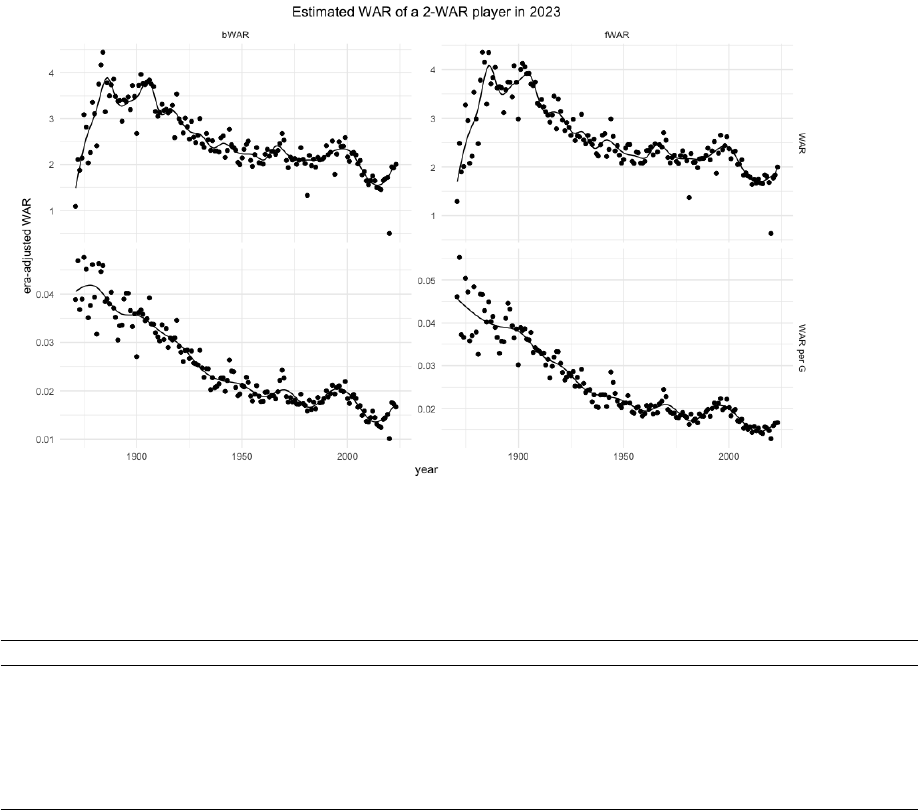
Figure 5: The ﬁgure in the top left shows the estimated bWAR values over time corresponding to a hypothetical player

with 2 bWAR in 2023; The ﬁgure in the top right shows the estimated fWAR values over time corresponding to a

hypothetical player with 2 fWAR in 2023; The ﬁgure in the bottom left shows the estimated bWAR per game values over

time corresponding to a hypothetical player with 2 bWAR in 2023; The ﬁgure in the bottom right shows the estimated

fWAR values over time corresponding to a hypothetical player with 2 fWAR in 2023. Note that there were fewer games

played in the early years of baseball.

name year AB per HR diﬀ Y

⋆⋆

balance n pBeta N X

Babe Ruth 1919 10.95 0.0662 0.00108 0.968 118 0.969 2020530 5355122

Babe Ruth 1920 10.88 0.0508 0.00040 0.985 130 0.985 2517182 12061976

Babe Ruth 1926 10.83 0.0413 0.00071 0.967 130 0.967 3499956 8272038

Barry Bonds 2001 10.86 0.0662 0.00140 0.959 243 0.960 11200119 18901295

Barry Bonds 2002 10.83 0.0259 0.00132 0.907 244 0.912 11725596 9660871

Barry Bonds 2004 10.76 0.0373 0.00161 0.920 242 0.924 12829045 11901386

Table 5: Comparison of the top three era-adjusted seasons by Babe Ruth and Barry Bonds according to home run rate

(AB per HR). N is the size of the talent pool, n is the number of full time players, Y

⋆⋆

is the upper bound calculated in

Section 2.2.3, and all other quantities are deﬁned in Section 4.1. Note that the absolute diﬀerence between the estimated

talent scores in the X appears large, but they are quite small when mapped to Pareto percentiles.

and efJAWS) ranking lists for each of the considered talent pool estimates. Talent pools B-C

yield similar results as our original talent pool with slight gains made by older era players. The

results yielded by talent pool D clearly favor older era players more than those yielded by talent

pools A-C. Talent pool E is the most favorable to older era players with Babe Ruth distancing

himself from the ﬁeld, and Cap Anson appearing ﬁrmly in the top 10. Note that Cap Anson’s

eJAWS is elevated by an increase in games played in the number of games that he likely would

play in our common mapping environment for comparing players (1977-1989 NL seasons with

the 1981 strike-shortened season removed).

Figure 6: Tail probability model ﬁts for home run rates for the top three era-adjusted seasons by Babe Ruth and Barry

Bonds according to home run rate.

5.2 Speciﬁcation that the most talented people are in the MLB

In this section, we perform a sensitivity analysis on our assumption that the most talented players

in the MLB. For example, it could be possible that our MLB interest adjustment may not capture

dual-sport athletes such as Kyler Murray and Pat Mahomes who are currently playing in the

NFL but might be among the most talented baseball players.

In this sensitivity analysis, we will suppose that the 10th, 20th, ..., and 100th talented

potential baseball players fail to start their sports career in baseball, which indicates the player

with the 10th largest bWAR or fWAR is paired with the 11th largest talent, the player with 20th

largest bWAR or fWAR is paired with 22nd largest talent, and so on. Then we mapped their

talents into the common mapping environment we built before and computed the era-adjusted

bWAR and fWAR. We perform this analysis for the seasons after the 1950 season corresponding

to a potential eﬀect due to the collapse of the Minor Leagues. We will also perform this analysis

for the seasons after the 1994 season based on the eﬀect of the MLB strike which saw the World

Series get canceled.

Table 7 shows the era-adjusted JAWS (eJAWS) rankings computed with respect to the 10th,

20th, ..., and 100th talented potential baseball players who fail to start their sports career in

baseball. The ranking of the top 10 is stable. After the top 10, we do see modern players

A B C D E

name eJAWS name eJAWS name eJAWS name eJAWS name eJAWS

1 Barry Bonds 106.17 Barry Bonds 106.47 Willie Mays 106.10 Babe Ruth 112.24 Babe Ruth 117.14

2 Roger Clemens 105.50 Roger Clemens 104.84 Babe Ruth 105.83 Barry Bonds 106.50 Ty Cobb 108.87

3 Willie Mays 101.94 Willie Mays 104.02 Barry Bonds 105.22 Roger Clemens 104.35 Willie Mays 107.51

4 Babe Ruth 95.50 Babe Ruth 100.28 Roger Clemens 103.36 Willie Mays 104.19 Barry Bonds 106.98

5 Henry Aaron 92.32 Henry Aaron 94.03 Henry Aaron 97.05 Ty Cobb 100.51 Cy Young 106.41

6 Alex Rodriguez 88.00 Stan Musial 88.33 Ty Cobb 92.31 Walter Johnson 95.29 Roger Clemens 105.75

7 Greg Maddux 87.06 Alex Rodriguez 87.46 Stan Musial 91.79 Henry Aaron 93.98 Cap Anson 105.38

8 Randy Johnson 86.99 Greg Maddux 86.28 Lefty Grove 89.54 Stan Musial 93.94 Walter Johnson 104.81

9 Stan Musial 86.00 Randy Johnson 86.07 Ted Williams 87.53 Lefty Grove 92.66 Honus Wagner 101.93

10 Mike Schmidt 83.37 Ty Cobb 86.04 Alex Rodriguez 85.84 Honus Wagner 91.15 Henry Aaron 98.54

11 Ted Williams 83.13 Ted Williams 85.27 Walter Johnson 85.74 Tris Speaker 90.48 Stan Musial 98.13

12 Lefty Grove 81.91 Lefty Grove 85.18 Greg Maddux 84.66 Cy Young 89.53 Tris Speaker 97.72

13 Albert Pujols 81.07 Mike Schmidt 83.93 Mike Schmidt 84.41 Ted Williams 89.32 Lefty Grove 93.98

14 Ty Cobb 80.74 Rickey Henderson 79.86 Randy Johnson 84.18 Rogers Hornsby 88.20 Eddie Collins 93.82

15 Rickey Henderson 80.48 Albert Pujols 79.37 Rogers Hornsby 83.75 Alex Rodriguez 87.94 Ted Williams 92.09

16 Justin Verlander 77.82 Rogers Hornsby 79.16 Tris Speaker 82.72 Greg Maddux 86.59 Rogers Hornsby 92.03

17 Joe Morgan 77.08 Joe Morgan 78.39 Lou Gehrig 81.15 Randy Johnson 85.56 Nap Lajoie 88.60

18 Cal Ripken Jr 75.58 Walter Johnson 77.96 Joe Morgan 79.84 Eddie Collins 85.07 Greg Maddux 87.34

19 Mike Trout 75.58 Tris Speaker 77.37 Mel Ott 79.75 Mel Ott 84.97 Randy Johnson 86.86

20 Rogers Hornsby 75.45 Lou Gehrig 77.31 Honus Wagner 79.60 Lou Gehrig 84.77 Mel Ott 86.76

21 Bert Blyleven 75.06 Justin Verlander 76.57 Rickey Henderson 78.68 Mike Schmidt 83.19 Lou Gehrig 86.27

22 Lou Gehrig 74.56 Mickey Mantle 76.25 Mickey Mantle 78.68 Cap Anson 81.33 Alex Rodriguez 85.12

23 Mickey Mantle 74.40 Mike Trout 75.43 Tom Seaver 76.67 Albert Pujols 81.03 Pete Alexander 83.86

24 Steve Carlton 74.40 Bert Blyleven 75.43 Steve Carlton 76.54 Rickey Henderson 80.28 Mike Schmidt 83.62

25 Tom Seaver 74.15 Steve Carlton 75.33 Frank Robinson 76.46 Jimmie Foxx 78.52 Mickey Mantle 83.50

Table 6: Era-adjusted JAWS (eJAWS) rankings computed with respect to talent pool estimates A-E. eJAWS is the aver-

age of era-adjusted JAWS computed using bWAR (ebJAWS), and era-adjusted JAWS computed using fWAR (efJAWS).

JAWS is the average of a players’ career WAR and the a players’ total WAR from his seven best seasons.

beginning to take a hit. For example, Albert Pujols ranks 13th in our original analysis, and he

falls slightly when some people who may have had better seasons than him are removed from

the talent pool. The eﬀect of the sensitivity analysis is most apparent for Mike Trout and Justin

Verlander who are active MLB players at the time this was written. These players drop out of

the top 25 list completely when very talented people are completely removed from the pool.

Original analysis Remove after 1950 Remove after 1994

name eJAWS name eJAWS name eJAWS

1 Barry Bonds 106.17 Barry Bonds 105.90 Barry Bonds 106.03

2 Roger Clemens 105.50 Roger Clemens 104.96 Roger Clemens 105.15

3 Willie Mays 101.94 Willie Mays 101.72 Willie Mays 102.08

4 Babe Ruth 95.50 Babe Ruth 95.50 Babe Ruth 95.50

5 Henry Aaron 92.32 Henry Aaron 91.54 Henry Aaron 92.24

6 Alex Rodriguez 88.00 Alex Rodriguez 87.39 Alex Rodriguez 87.39

7 Greg Maddux 87.06 Randy Johnson 86.09 Randy Johnson 86.65

8 Randy Johnson 86.99 Greg Maddux 85.75 Greg Maddux 86.46

9 Stan Musial 86.00 Stan Musial 84.79 Stan Musial 85.85

10 Mike Schmidt 83.36 Mike Schmidt 83.05 Mike Schmidt 83.37

11 Ted Williams 83.13 Ted Williams 82.88 Ted Williams 83.18

12 Lefty Grove 81.91 Lefty Grove 81.91 Lefty Grove 81.91

13 Albert Pujols 81.06 Ty Cobb 80.72 Ty Cobb 80.72

14 Ty Cobb 80.74 Rickey Henderson 79.13 Rickey Henderson 79.38

15 Rickey Henderson 80.48 Albert Pujols 78.84 Albert Pujols 78.84

16 Justin Verlander 77.82 Joe Morgan 76.00 Joe Morgan 77.09

17 Joe Morgan 77.09 Rogers Hornsby 75.44 Rogers Hornsby 75.44

18 Cal Ripken Jr 75.58 Lou Gehrig 74.56 Bert Blyleven 75.06

19 Mike Trout 75.58 Cal Ripken Jr 74.02 Cal Ripken Jr 74.81

20 Rogers Hornsby 75.44 Mickey Mantle 73.84 Lou Gehrig 74.56

21 Bert Blyleven 75.06 Bert Blyleven 73.78 Mickey Mantle 74.41

22 Lou Gehrig 74.56 Tom Seaver 73.05 Steve Carlton 74.40

23 Mickey Mantle 74.40 Steve Carlton 72.97 Tom Seaver 74.13

24 Steve Carlton 74.40 Wade Boggs 72.65 Wade Boggs 73.05

25 Tom Seaver 74.15 Mel Ott 72.64 Mel Ott 72.64

Table 7: Era-adjusted JAWS (eJAWS) rankings computed with respect to the 10th, 20th, ..., and 100th most talented

potential baseball players not being in the MLB for every season after some stated season (1950 and 1994). eJAWS is

the average of era-adjusted JAWS computed using bWAR (ebJAWS), and era-adjusted JAWS computed using fWAR

(efJAWS). JAWS is the average of a player’s career WAR and the player’s total WAR from his seven best seasons. The

original analysis is our top 25 JAWS list without removing players.

5.3 Multiverse Analyses

We investigate how modeling choices can aﬀect results through two comparisons using a multi-

verse analytical approach Steegen et al. [2016]. The ﬁrst comparison is made with respect to the

batting averages of 1997 Tony Gwynn and 1911 Ty Cobb. The second comparison is made with

respect to the at-bats per home run of 2001 Barry Bonds and 1920 Babe Ruth.

Four modeling choices were considered: the park-factor eﬀect, the eﬀect of the talent pool,

whether or not the distribution of the batting statistics is parametric or nonparametric (only

relevant for batting average comparisons, the parametric distribution for batting averages is the

normal distribution), and the number of full-time players.

The modeling choices have a more pronounced impact on our batting average comparison than

our AB per home run comparison. We also note that in this comparison of batting averages

we see that the modeling choice used in our analysis (park-factor = YES; Talent Pool = A;

Distribution = nonparametric; League Size = historical) is the most favorable conﬁguration for

1997 Tony Gwynn relative to 1911 Ty Cobb. See the Supplementary Materials for more details.

6 Summary and Discussion

Michael Schell went to great lengths to compare batters across eras in two books, Schell [1999]

and Schell [2005]. Motivated by Gould [1996], Schell also considered the standard deviation as

a proxy for measuring a changing talent pool. On page 58 in Schell [2005], he outlined some

problems with his standard deviation approach and called for a more sophisticated statistical

method to handle diﬃculties with the changing talent pool. He said: “Someday we will need to

abandon the use of the standard deviation as a talent pool adjustment altogether and search for

another talent pool adjustment method, likely involving more diﬃcult statistical methods than

those used in this book.” Our work answers Schell’s call through the development of a novel

statistical model which directly connects achievement to talent after a careful estimate of the

size of the talent pool is supplied as a modeling input.

Estimation the talent pool comes with some level of subjectivity, and diﬀerent estimates of

the talent pool can yield diﬀerent results. This can be seen in Section 5.1 where we consider

results based alternative talent pool estimates, labeled B-E. We provide some reasons for the

shortcomings of each of these alternative talent pools. Baseball interest as deﬁned in B and C

above yield an estimated talent pool that is not alignment with a talent pool constructed from

Latin American countries (details are at the end of the linked report included in Section 3.1).

Talent pool D corresponds to the erosion of the Minor Leagues following their peak in 1949

It is speculated that this collapse of the Minor Leagues led to an increase in MLB competitive

balance because potentially exceptional players were lost due to professional baseball opportuni-

ties being removed (see the last paragraph of the Discussion in Horowitz [1997]). Furthermore,

it is occasionally speculated that this collapse was during a time in which baseball was thought

of as an avenue for elevating the social status of lower-income men. However, the Minor League

teams that were lost were lower quality teams, a majority of which were not aﬃliated with MLB

farm systems [Land et al., 1994]. Sullivan [1990] attributed the decline in the minor leagues to

https://www.milb.com/milb/history/general-history

relocation of MLB teams to Minor League markets and the spread of television broadcasting

games. Bellamy and Walker [2004] noted that television went from 0.4 percent of U.S. house-

holds in 1948 to 87.1 percent in 1960. However, these authors concluded that “the extension

of MLB radio broadcasts, both national and local, in combination with a market correction,

probably hurt the Minor Leagues, particularly in the ﬁrst half of the 1950s, much more than

the televised broadcasts that were in their infancy.” Riess [1980] studied professional baseball

and social mobility in the Progressive era. He concluded that professional baseball was “greatly

overrated as a source of upward mobility when the game was at its unchallenged height.” In

aggregate, we argue that our original talent pool estimate is more sensible than talent pool D,

but we understand if the reader disagrees. Talent pool E is constant over time and therefore

ignores the history of westward and southern expansion of baseball, integration, globalization,

and eﬀects of war, etc. Estimation of the talent pool is a research area of its own. Changing

player salaries, changing media environments, demographic-speciﬁc interest in baseball, and the

mechanisms by which international talent joins the MLB could all be avenues for improving the

estimate of the talent pool.

Importantly, we found that several great non-white and non-American players sit atop the

era-adjusted WAR rankings. This is due to increased inclusion and general population increases

in the talent pool over time. Our analyses found that more modern players such as Barry Bonds

and Willie Mays have better careers than the legendary Babe Ruth. Current players to the

time of this writing are adding legendary seasons to baseball’s storied history. In particular, we

highlight Shohei Ohtani and Aaron Judge’s 2022 campaign, and Mike Trout’s recent stretch of

great seasons. All-time great baseball is being played right now, and we are excited for what the

future holds. We are conﬁdent that this will remain true at the time you are reading this paper.

Supplementary Materials

This article is accompanied by an extensive set of Supplementary Materials. First, there is a

traditional supplement that complements this submission. There is also a GitHub repository

containing further analyses and reports. This repository can be viewed here:

https://github.com/ecklab/era-adjustment-app-supplement.

We have also created a website that contains era-adjusted statistics for all qualifying baseball

players from 1871-2023. This website includes a top 100 list by career ebWAR and efWAR as

well as player pages that include era-adjusted and unadjusted statistics. This website can be

viewed here:

https://eckeraadjustment.web.illinois.edu/

Acknowledgments

We are also grateful to Mark Armour, Forrest W. Crawford, David Dalpiaz, Adam Darowski,

Louis Moore, Ben Sherwood, Sihai Dave Zhao, and many others for helpful comments and great

discussions.

Supplementary Materials for Comparing baseball players

across Eras via the Novel Full House Model

This Supplementary Material includes:

• Pre-processing steps that were made for batting and pitching statistics.

• An investigation into the often-referenced claim that batting averages for full-time players

are normally distributed.

• Additional sensitivity analyses for modeling assumptions.

• A visualization of the common-mapping environment used to compute era-adjusted bWAR

for batters.

• Multiverse Analyses comparing the batting averages of 1997 Tony Gwynn and 1911 Ty

Cobb, the at-bats per home run of 2001 Barry Bonds and 1920 Babe Ruth, top 25 career

batting averages and top 25 four-year peaks by batting average.

• Brief theoretical details of

(t), as deﬁned in equation (3) in the manuscript.

More materials can be seen on our GitHub repository:

https://github.com/ecklab/era-adjustment-app-supplement

This GitHub repository contains a detailed write-up on our estimation of the talent pool,

codes for scrapping data from Baseball-Reference and Fangraphs, codes for the pre-process of

batting and pitching stats, and a reproducible technical report that reproduces important tables

and ﬁgures.

7 Pre-prossesing of batting and pitching statistics

7.0.1 Batting statistics

In this section, we detail the considerations made for the batting statistics that we era-adjust

using our methodology: batting average (BA), hits (H), home runs (HR), walks (BB), on-base

percentage (OBP), bWAR, and fWAR. These statistics are all modeled on a rate basis where

count statistics are converted to rates: we model HR/AB, BB/PA, bWAR/G, and fWAR/G. We

also adjust at-bats (AB) and plate appearances (PA) to accommodate changing season lengths

throughout baseball’s history. Handedness-speciﬁc park factor adjustments are also considered

for BA and HR in our model. We apply the adjusted park index from Schell [2005] to all ballparks

from 1871-2023. We use nonparametric methods to model all statistics since these statistics (with

the possible exception of BA) have not been demonstrated to follow any common distribution

that we know.

Our modeling will only be applied to full-time batters. We deﬁne full-time batters as anyone

above the median number of PAs after screening out hitters who appeared in fewer than 75 PAs.

This criterion is ﬂexible enough to account for changing the number of games played over time as

well as seasons shortened by labor strikes and pandemics. To deal with extreme statistics from

the small sample size, we employed a shrinkage method that adjusted the raw statistics toward

a global average. Our shrinkage method follows a shrinkage of team ballpark eﬀect estimates

motivated from Schell [2005]. The Schell [2005] method involved the weighted average of raw

components (hits, home runs, etc.) for total team statistics of the form

adjusted statistic =

raw statistic × total ABs + 4000 × league average of the statistic

(total ABs + 4000)

This shrinkage method from Schell [2005] will shrink the team average to the league average.

In our context of shrinkage for individual player statistics, we change the shrinkage factor

4000

totals AB + 4000

. For example, our shrinkage factor for bWAR per game is

individual games + 7

The ratio

individual games + 7

is approximately equal to

4000

totals AB + 4000

. Thus,

adjusted bWAR per game =

raw bWAR per game × individual games + 7 × league average bWAR per game

individual games + 7

We calculate mapped games and plate appearances by applying quantile mapping. Quantile

mapping is based on the idea that a pth percentile player’s games in one year are equal to a pth

percentile player’s games in another year. AB and PA also change across baseball history as the

number of games and walk rates change. We calculate adjusted AB as:

adjusted AB = adjusted PA - adjusted BB - HBP - SH - SF, (8)

where HBP, SH, and SF are short for, respectively, hit by pitch, sacriﬁce hits, and sacriﬁce ﬂies,

and adjusted PA is a player’s quantile-mapped PA total from the season under study to that

in the common-mapping environment (NL seasons from 1977 through 1989, excluding the 1981

strike-shortened season).

From here, era-adjusted hits, walks, and home runs can be computed from the per AB rates

and (8) and adjusted PAs. For example, era-adjusted hits is equal to era-adjusted batting average

multiplied by adjusted AB. Era-adjusted bWAR (ebWAR) or fWAR (efWAR) are obtained by

multiplying era-adjusted bWAR per game or fWAR per game with adjusted games. We also

compute era-adjusted OBP as

era-adjusted OBP =

era-adjusted BA * adjusted AB + era-adjusted BB + HBP

adjusted AB + era-adjusted BB + HBP + SF

. (9)

We ﬁnd that the Full House Model can harshly punish the tails of players’ careers, especially

for older-era players. This is due to players reaching or staying in the MLB during a less talented

era of baseball history, and having these seasons translates to terrible play in the common context

that we judge all players. For example, a late-career decline in the 1910s would correspond to

a player who would likely be out of the MLB in the 1980s. We eliminate players who had an

era-adjusted bWAR (ebWAR) or era-adjusted fWAR (efWAR) below the replacement level for

more than half of their career seasons. We also set three rules to eliminate some players’ poor

early and late career seasons. The three rules are: 1) in at least 2 consecutive seasons, the

ebWAR is below -1.5; 2) in at least 2 consecutive seasons, the efWAR is below -1.5; 3) in at least

two consecutive seasons, no more than one ebWAR or efWAR can be more than 0.2. The value

0.2 is calculated from the average ebWAR or efWAR of the players that disappeared from the

MLB from the 1977 season to the 1989 season with the exception of the 1981 strike-shortened

season.

7.0.2 Pitching statistics

In this section, we detail the considerations made for the pitching statistics that we era-adjust

using our methodology: earned-run average (ERA), strikeouts (SO), bWAR, and fWAR. We also

adjust innings pitched (IP) using a similar quantile mapping approach that we applied to games

or PA for batters. We will use nonparametric methods to measure these pitching statistics since

these statistics have not been demonstrated to follow any common distribution we know. Note

that smaller values of ERA are better, so we apply the Full House Model to the negation of ERA.

Career trimming and shrinkage were applied to era-adjusted pitching statistics in the same way

as to batting statistics.

Our modeling will only be applied to full-time pitchers. We deﬁne full-time pitchers as the n

pitchers who pitched the most innings above a cutoﬀ. We now describe how the cutoﬀ is deﬁned:

we get the average rotation size for each time in the MLB, and then we add these rotation sizes

to arrive at n full-time pitchers.

8 Investigation of normality of batting averages

We initially tried parametric distributions to model BA since it is widely recognized that BA

follows a normal distribution [Gould, 1996]. We perform a Shapiro-Wilk test [Shapiro and Wilk,

1965] of normality on the BA distribution for each season. Table 8 shows the p-values from

the Shapiro-Wilk test for each season. Figure 7 shows the histogram of the p-values from the

Shapiro-Wilk test of normality on the BA distribution in each season. We observe that rejection

rates from Shaprio-Wilk tests exceed nominal thresholds. Thus we will utilize the nonparametric

distribution to measure the BA in each season because the normality of the BA distribution is

not consistent with the data.

threshold proportion of seasons exceeding threshold

0.05 0.15

0.1 0.24

0.2 0.34

0.3 0.39

Table 8: The table shows the percent of seasons in which BA failed the Shapiro-Wilk test based on diﬀerent p-value

thresholds.

Figure 7: Histogram of the p-values from Shapiro-Wilk test of normality on the BA distribution in each season.

9 Sensitivity analyses

In this section, we validate our model to ensure the appropriateness of the assumption that

the talent-generating process is Pareto distribution with parameter α = 1.16 via a sensitivity

analysis simulation. The goal of this analysis is to determine how many of the top 25 talented

players by BA our method can correctly identify under a variety of simulation conﬁgurations,

some of which are chosen to stretch the credibility of our method.

In each simulation, we ﬁrst randomly generate samples from four diﬀerent talent generation

distributions, which are the Pareto distribution with parameter α = 1.16 (i.e. the talent gen-

erating process is correctly speciﬁed), Pareto distribution with parameter α = 3, folded normal

distribution with parameters µ = 0, σ = 1, and standard normal distribution. Within each talent

generation distribution, we vary the talent pool sizes N

for ﬁve diﬀerent hypothetical leagues.

Details of the simulation information are in Table 9.

league sample size µ σ improved estimation deteriorated estimation

1 1 ∗ 10

0.280 0.040 0.5 ∗ 10

1 ∗ 10

2 2 ∗ 10

0.275 0.0375 1.5 ∗10

1 ∗ 10

3 4 ∗ 10

0.270 0.035 3.33 ∗10

1.33 ∗ 10

4 8 ∗ 10

0.265 0.0325 7 ∗ 10

2 ∗ 10

5 16 ∗ 10

0.260 0.030 14.4 ∗10

3.2 ∗ 10

Table 9: Simulation study conﬁgurations. The sample size represents the talent pool for each of the ﬁve leagues. µ and

σ are the parameters of the normal distribution for generated batting averages. The improved estimation column is the

estimated talent pool where the estimation improves. The deteriorated estimation column is the estimated talent pool

where the estimation deteriorates.

Then we select 300 people with the largest talents in each dataset and consider them as

the full-time batters in MLB. Therefore, n

= 300 for all i. We will generate BA from the

talent scores using a normal distribution with parameters Table 9. For each league i, these

values are generated as Y

i,(j)

= F

−1



−1

i,(j)



i,(N

−n

+j)

i,N

−n

)



|θ



, where θ

are the

parameters for the normal distribution, and our choices for these parameters reﬂect the shrinking

BA variability that has been observed over time [Gould, 1996].

We apply the Full House Model with F

assumed to be Pareto with α = 1.16 to this generated

data and investigate how well the Full House Model correctly identiﬁes the top 25 players as

judged by talent scores. We also consider misspeciﬁcation in the estimation of the talent pool

size.

We consider two underestimations of the talent pool where 1) the estimation improves as

time increases and 2) the underestimation deteriorates as time increases. This conﬁguration

was chosen to be deliberately antagonistic to our method, especially when the talent-generating

process was misspeciﬁed. The details of the information are in Table 9. We also compare our

Full House Model to rankings based on Z-scores and unadjusted BA. Z-scores are a building

block for the Power Transformation Method method.

200 Monte Carlo iterations of our simulation are performed and the results are depicted in

Figure 8 and Table 10.

What we found is that our Pareto assumption with α = 1.16 holds up well even when the

talent-generating process and the talent pool is not correctly speciﬁed. Moreover, our method

correctly identiﬁes more top-25 talented players than both Z-scores and raw unadjusted batting

averages.

That being said, there is considerable overlap between the box plot in the second row and

the box plot in the fourth row. This suggests that Z-scores may not be strictly worse than our

method under misspeciﬁcation. A more detailed look shows that this is not the case. During

Figure 8: Monte Carlo simulation investigating the number of correctly identiﬁed talents in a top 25 list under four

diﬀerent latent talent distribution F

. Each column of the plot indicates a diﬀerent talent generation distribution. The

ﬁrst three rows of the plot are variants of our Full House Model where F

is assumed to be Pareto with α = 1.16. The

ﬁrst row displays the performance of our method with the talent pool correctly estimated. The second and third rows

display the performance of our method with the talent pool incorrectly estimated. In the second row, we underestimate

the talent pool where the estimation improves as the talent pool increases. In the third row, we underestimate the talent

pool where the estimation deteriorates as the talent pool increases. The fourth row displays the performance of Z-scores

and the ﬁfth row displays the performance of raw unadjusted batting averages.

each simulation, we directly compare our method when the underestimation estimation of the

talent pool deteriorates and Z-scores (third and fourth rows of Figure 8). Then we calculate the

proportion of simulations that our model with the population estimation deteriorates strictly

beats the Z-scores method and either beats or ties the Z-scores method. Table 10 indicates that

our Full House Model is almost strictly better than the Z-scores method in each simulation.

Thus, the Full House Model performs better than Z-scores even when F

and the estimated

eligible population sizes are badly misspeciﬁed.

Correct Pareto distribution Incorrect Pareto distribution Normal distribution Folded normal distribution

beats or ties 1 1 1 1

strictly beats 1 1 0.995 1

Table 10: Comparison of results between rows 3 and 4 of Figure 8. The columns display the talent-generating distribution.

The entries of the table display the proportion of Monte Carlo iterations for which the Full House Model with assumed

Pareto talent generating process with α = 1.16 and the talent pool estimated via the deteriorated estimation regime

(see Table 9) strictly beats or ties Z-scores in the number of top 25 talents correctly identiﬁed.

We validate the stability of rankings when we change the latent distribution F

to a folded

normal distribution, the Pareto distribution with α = 3, and the standard normal distribution.

Table 11 shows the rankings with these three diﬀerent latent talent distributions. As expected,

the distribution assumed on F

does not inﬂuence the results.

Standard normal Folded normal (µ = 0, σ = 1) Pareto with α = 3 Pareto with α = 1.16

name ebWAR name ebWAR name ebWAR name ebWAR

1 Barry Bonds 153.9 Barry Bonds 153.9 Barry Bonds 153.9 Barry Bonds 153.9

2 Roger Clemens 145.91 Roger Clemens 145.91 Roger Clemens 145.91 Roger Clemens 145.91

3 Willie Mays 144.1 Willie Mays 144.1 Willie Mays 144.1 Willie Mays 144.1

4 Henry Aaron 135.6 Henry Aaron 135.6 Henry Aaron 135.6 Henry Aaron 135.6

5 Babe Ruth 132.7 Babe Ruth 132.7 Babe Ruth 132.7 Babe Ruth 132.7

6 Stan Musial 119.51 Stan Musial 119.51 Stan Musial 119.51 Stan Musial 119.51

7 Alex Rodriguez 119.07 Alex Rodriguez 119.07 Alex Rodriguez 119.07 Alex Rodriguez 119.07

8 Greg Maddux 113.67 Greg Maddux 113.67 Greg Maddux 113.67 Greg Maddux 113.67

9 Ty Cobb 112 Ty Cobb 112 Ty Cobb 112 Ty Cobb 112

10 Albert Pujols 111.85 Albert Pujols 111.85 Albert Pujols 111.85 Albert Pujols 111.85

11 Randy Johnson 110.81 Randy Johnson 110.81 Randy Johnson 110.81 Randy Johnson 110.81

12 Mike Schmidt 109.59 Mike Schmidt 109.59 Mike Schmidt 109.59 Mike Schmidt 109.59

13 Rickey Henderson 109.06 Rickey Henderson 109.06 Rickey Henderson 109.06 Rickey Henderson 109.06

14 Ted Williams 108.04 Ted Williams 108.04 Ted Williams 108.04 Ted Williams 108.04

15 Tom Seaver 104.31 Tom Seaver 104.31 Tom Seaver 104.31 Tom Seaver 104.31

16 Lefty Grove 101.58 Lefty Grove 101.58 Lefty Grove 101.58 Lefty Grove 101.58

17 Tris Speaker 100.7 Tris Speaker 100.7 Tris Speaker 100.7 Tris Speaker 100.7

18 Justin Verlander 100.24 Justin Verlander 100.24 Justin Verlander 100.24 Justin Verlander 100.24

19 Joe Morgan 100.17 Joe Morgan 100.17 Joe Morgan 100.17 Joe Morgan 100.17

20 Frank Robinson 99.91 Frank Robinson 99.91 Frank Robinson 99.91 Frank Robinson 99.91

21 Bert Blyleven 97.69 Bert Blyleven 97.69 Bert Blyleven 97.69 Bert Blyleven 97.69

22 Cal Ripken Jr 97.41 Cal Ripken Jr 97.41 Cal Ripken Jr 97.41 Cal Ripken Jr 97.41

23 Mel Ott 96.72 Mel Ott 96.72 Mel Ott 96.72 Mel Ott 96.72

24 Rogers Hornsby 95.76 Rogers Hornsby 95.76 Rogers Hornsby 95.76 Rogers Hornsby 95.76

25 Lou Gehrig 95.68 Lou Gehrig 95.68 Lou Gehrig 95.68 Lou Gehrig 95.68

Table 11: ebWAR rankings from Full House Model using diﬀerent latent talent distributions: Standard normal, Folded

normal (µ = 0, σ = 1), Pareto with α = 3, and Pareto with α = 1.16.

10 Isotonic Regression for Common-Mapping Environment

Figure 9 shows the relationship between bWAR talent and bWAR per game. The black dots

represent the observations from the full-time batters from the 1977 season to the 1989 season

except for the 1981 strike-shortened season. The red dots represent the observations from the

common mapping environment that we deﬁne in the manuscript. Based on the ﬁgure above, the

observations from the common mapping environment accurately depict the relationship between

bWAR talent and bWAR per game from the 1977 season to the 1989 season except for the 1981

strike-shortened season.

11 Pairings of the maximum talent scores with their cor-

responding era-adjusted bWAR for players in the com-

mon mapping environment

Figure 10 shows the pairings of the maximum talent scores with their corresponding era-adjusted

bWAR for players in the common mapping environment. The X-axis is their bWAR talent and

Figure 9: The relationship between bWAR talent and bWAR per game. The black dots represent the observations from

the full-time batters from the 1977 season to the 1989 season except for the 1981 strike-shortened season. The red dots

represent the observations from the common mapping environment that we deﬁne in the manuscript. The talent values

are computed using displayed equation (4) in the manuscript where y

⋆⋆

is computed in displayed equation (5) in the

manuscript.

the Y-axis is their corresponding era-adjusted bWAR. Note that the the y

⋆⋆

value for bWAR

per game in the common-mapping environment is 0.00325, and that Lonnie Smith’s 1989 season

ranked 116th overall.

12 Multiverse Analyses

In this section, we will show how modeling choices can aﬀect results through two comparisons.

The ﬁrst comparison is made with respect to the batting averages of 1997 Tony Gwynn and 1911

Ty Cobb. The second comparison is made with respect to the at-bats per home run of 2001

Barry Bonds and 1920 Babe Ruth.

The four modeling choices considered are the park-factor eﬀect, the talent pool, whether

or not the distribution of the batting statistics is parametric or nonparametric (only relevant

for batting average comparisons, the parametric distribution for batting averages is the normal

distribution), and the number of full-time players.

Results are displayed in Table 12 and Table 13. The modeling choices have a more pro-

nounced impact on the batting average comparison than the AB per home run comparison.

When comparing batting averages we see that the modeling choice used in our analysis (park-

Figure 10: The pairings of the maximum talent scores with their corresponding era-adjusted bWAR for players in the

common mapping environment. The X-axis is their bWAR talent and the y-axis is their corresponding era-adjusted

bWAR.

factor = YES; Talent Pool = A; Distribution = nonparametric; League Size = historical) is the

most favorable conﬁguration for 1997 Tony Gwynn relative to 1911 Ty Cobb. We argue for talent

pool A in the manuscript, use a handedness-speciﬁc park-factor method used by Schell [2005],

and have demonstrated in this supplement that the normal distribution might be inappropriate

as a model for batting averages. We think our modeling choices are sensible, but understand if

the reader disagrees.

We also show how the distribution of the batting statistics can aﬀect the overall batting

average results. Table 14 shows the distribution of the batting statistics aﬀects the top 25 career

batting averages and top 25 four-year peaks by batting average.

Stephen Jay Gould

suggests that the BA in every season follows a normal distribution

[Gould, 1996] and we perform the Shapiro-Wilk Normality Test to verify this argument. The

details are under Section 8 and we found the BAs do not follow the normal distribution for a

signiﬁcant proportion of seasons. So we use the nonparametric method to measure the BAs. We

understand if the reader disagrees.

https://en.wikipedia.org/wiki/Full_House:_The_Spread_of_Excellence_from_Plato_to_Darwin

13 Theoretical Results

In the main text it was noted that

(t) was explicitly constructed to be close to

(t). We

now formalize this statement.

Proposition 13.1. Let

(t) be deﬁned as in (2) and let

(t) be the empirical distribution

function. Then, sup

t∈R



(t) −

(t)



≤

Proof. We will prove this result in cases. First, when t ≤

i,(1)

or t ≥

i,(n+1)

we have that

(t)−

(t) |= 0. For any j = 1, . . . , n and

i,(j)

≤ t < Y

i,(j)

, we have



(t) −

(t)



j −1

−

j −1 +



t −

i,(j)





i,(j+1)

−

i,(j)





≤

For any j = 1, . . . , n and Y

i,(j)

< t <

i,(j+1)

, we have



(t) −

(t)



−

j −1 +



t −

i,(j)





i,(j+1)

−

i,(j)





≤

Our conclusion follows.

This leads to a Glivenko-Cantelli result which is appropriate for

Corollary 13.1.1. Let

(t) be deﬁned as in (1) and let

(t) be the empirical distribution

function. Then, sup

t∈R



(t) − F

(t)



a.s

−→ 0.

Proof. We have, sup

t∈R



(t) − F

(t)



≤ sup

t∈R



(t) −

(t)



+sup

t∈R



(t) − F

(t)



. The

conclusion follows from the Glivenko-Cantelli Theorem and Proposition 2.1.

References

J. Albert and J. Bennett. Curve Ball: Baseball, Statistics, and the Role of Chance in the Game.

Copernicus Books, 2003.

M. Armour. The Eﬀects of Integration, 1947–1986. The Baseball Research Journal, 36:53–57,

2007.

M. Armour and D. R. Levitt. Baseball Demographics, 1947–2016. Society for American Baseball

Research, 2016.

Baseball Prospectus Staﬀ. WARP. 2013. URL http://www.baseballprospectus.com/

glossary/.

B. S. Baumer and G. J. Matthews. A statistician reads the sports page: There is no avoiding

WAR. Chance, 27(3):41–44, 2014.

B. S. Baumer, S. T. Jensen, and G. J. Matthews. openWAR: An open source system for eval-

uating overall player performance in major league baseball. Journal of Quantitative Analysis

in Sports, 11(2):69–84, 2015.

R. V. Bellamy and J. R. Walker. Did Televised Baseball Kill the ”Golden Age” of the Minor

Leagues? NINE: A Journal of Baseball History and Culture, 13(1):59–73, 2004.

D. Berri and M. Schmidt. Stumbling on Wins (Bonus Content Edition): Two Economists Expose

the Pitfalls on the Road to Victory in Professional Sports, Portable Documents. Pearson

Education, 2010.

S. M. Berry, C. S. Reese, and P. D. Larkey. Bridging diﬀerent eras in sports. Journal of the

American Statistical Association, 94(447):661–676, 1999.

B. Bullpen. Wins Above Replacement. 2023. URL "https://www.baseball-reference.com/

bullpen/Wins_Above_Replacement".

A. Burgos Jr. Playing America’s Game. University of California Press, 2007.

D. J. Eck. Challenging nostalgia and performance metrics in baseball. Chance, 33(1):16–25,

2020a.

D. J. Eck. Challenging WAR and Other Statistics as Era-Adjustment

Tools. FanGraphs, 2020b. https://community.fangraphs.com/

challenging-war-and-other-statistics-as-era-adjustment-tools/.

ESPN. Top 100 MLB players of all time, 2022. URL https://www.espn.com/mlb/story/_/

id/33145121/top-100-mlb-players-all.

S. Forman. Player Wins Above Replacement. 2010. URL http://www.baseball-reference.

com/blog/archives/6063.

M. Friendly, C. Dalzell, M. Monkman, D. Murphy, V. Foot, J. Zaki-Azat, and S. Lahman. Lah-

man: Sean ’Lahman’ Baseball Database, 2023. URL https://CRAN.R-project.org/package=

Lahman. R package version 11.0-0.

S. J. Gould. Full House: The Spread of Excellence from Plato to Darwin. Harvard University

Press, 1996.

D. C. Hoaglin et al. Letter values: A set of selected order statistics. Understanding robust and

exploratory data analysis, pages 33–57, 1983.

I. Horowitz. The increasing competitive balance in Major League Baseball. Review of industrial

Organization, 12:373–387, 1997.

W. Kaczynski, L. Leemis, N. Loehr, and J. McQueston. Nonparametric random variate genera-

tion using a piecewise-linear cumulative distribution function. Communications in Statistics-

Simulation and Computation, 41(4):449–468, 2012.

K. C. Land, W. R. Davis, and J. R. Blau. Organizing the boys of summer: The evolution of US

minor-league baseball, 1883-1990. American Journal of Sociology, 100(3):781–813, 1994.

D. M. Leenaerts and W. M. V. Bokhoven. Piecewise Linear Modeling and Analysis. Kluwer

Academic Publishers, 1998.

M. Lewis. Moneyball: The art of winning an unfair game. WW Norton & Company, 2003.

V. McCracken. Pitching and defense: How much control do hurlers have? Baseball Prospectus,

23, 2001.

M. E. Newman. Power laws, Pareto distributions and Zipf’s law. Contemporary physics, 46(5):

323–351, 2005.

H. of Stats, 2022. URL http://hallofstats.com/.

V. Pareto. Cours d’

Economie Politique: Nouvelle ´edition par G.-H. Bousquet et G. Busino.

Librairie Droz, 1964.

J. Posnanski. The Baseball 100. Avid Reader Press, 2021.

B. G. Rader. Baseball: A history of America’s game (3rd edition). University of Illinois Press,

2008.

S. A. Riess. Professional baseball and social mobility. The Journal of Interdisciplinary History,

11(2):235–250, 1980.

M. J. Schell. Baseball’s all-time best hitters. Princeton University Press, 1999.

M. J. Schell. Baseball’s all-time best sluggers. Princeton University Press, 2005.

M. B. Schmidt and D. J. Berri. Concentration of playing talent: evolution in Major League

Baseball. Journal of Sports Economics, 6(4):412–419, 2005.

F. Scholz. Nonparametric tail extrapolation. White paper from Boeing Information & Support

Services) http://www. stat. washington. edu/fritz/Reports/ISSTECH-95-014. pdf, 1995.

S. S. Shapiro and M. B. Wilk. An analysis of variance test for normality (complete samples).

Biometrika, 52(3/4):591–611, 1965.

B. W. Silverman. Density estimation for statistics and data analysis, volume 26. CRC press,

1986.

P. Slowinski. What is WAR? FanGraphs, 2010. URL https://library.fangraphs.com/misc/

war/.

S. Steegen, F. Tuerlinckx, A. Gelman, and W. Vanpaemel. Increasing transparency through a

multiverse analysis. Perspectives on Psychological Science, 11(5):702–712, 2016.

M. L. Stein. A parametric model for distributions with ﬂexible behavior in both tails. Environ-

metrics, page e2658, 2020.

N. J. Sullivan. The Minors. Macmillan, 1990.

T. M. Tango, M. G. Lichtman, and A. E. Dolphin. The book: Playing the percentages in baseball.

Potomac Books, Inc., 2007.

J. Thorn and P. Palmer. The hidden game of baseball: A revolutionary approach to baseball and

its statistics. University of Chicago Press, 1984.

Park factor Talent pool Distribution League size Diﬀerence

YES A parametric historical 0.020

ﬁxed 0.008

nonparametric historical 0.040

ﬁxed 0.040

B parametric historical 0.017

ﬁxed 0.006

nonparametric historical 0.035

ﬁxed 0.035

C parametric historical 0.014

ﬁxed 0.003

nonparametric historical 0.023

ﬁxed 0.023

D parametric historical 0.010

ﬁxed -0.001

nonparametric historical 0.006

ﬁxed 0.006

E parametric historical 0.006

ﬁxed -0.005

nonparametric historical -0.002

ﬁxed -0.002

NO A parametric historical 0.005

ﬁxed 0.002

nonparametric historical 0.029

ﬁxed 0.029

B parametric historical 0.003

ﬁxed -0.001

nonparametric historical 0.027

ﬁxed 0.027

C parametric historical 0.000

ﬁxed -0.003

nonparametric historical 0.015

ﬁxed 0.015

D parametric historical -0.004

ﬁxed -0.008

nonparametric historical 0.007

ﬁxed 0.007

E parametric historical -0.007

ﬁxed -0.010

nonparametric historical -0.003

ﬁxed -0.003

Table 12: The table shows the value of the era-adjusted BA of Tony Gwynn in the 1997 season minus the era-adjusted

BA of Ty Cobb in the 1911 season under diﬀerent conﬁgurations. The Park factor column indicates whether we apply

the park-factor adjustment to the BA. The Talent pool column indicates the population changes we apply to the talent

pool. Population A - E are constructed according to the ﬁve diﬀerent estimates of the talent pool in Section 5 of

the manuscript. The Distribution column indicates we use parametric distribution and nonparametric distribution to

measure the BA in each season. The League size column indicates how full-time players are calculated. Historical means

that we use the number of full-time players observed for the given. Fixed means that the number of full-time players is

set to the maximum number of seasonal full-time players observed in our data set. The Diﬀerence indicates the value of

the BA of Tony Gwynn in the 1997 season minus the BA of Ty Cobb in the 1911 season under diﬀerent conﬁgurations.

Park factor Talent pool League size Diﬀerence

YES A historical -0.037

ﬁxed -0.037

B historical -0.012

ﬁxed -0.012

C historical 0.007

ﬁxed 0.007

D historical 0.020

ﬁxed 0.020

E historical 0.028

ﬁxed 0.028

NO A historical -0.010

ﬁxed -0.010

B historical 0.038

ﬁxed 0.038

C historical 0.084

ﬁxed 0.084

D historical 0.100

ﬁxed 0.100

E historical 0.100

ﬁxed 0.100

Table 13: The table shows the value of the era-adjusted AB per HR of Barry Bonds in the 2001 season minus the era-

adjusted AB per HR of Babe Ruth in the 1920 season under diﬀerent conﬁgurations. The Park factor column indicates

whether we apply the park-factor adjustment to the home run. The Talent pool column indicates the population changes

we apply to the talent pool. Population A - E are constructed according to the ﬁve diﬀerent estimates of the talent pool

in Section 5 of the manuscript. The League size column indicates how full-time players are calculated. Historical means

that we use the number of full-time players observed for the given. Fixed means that the number of full-time players is

set to the maximum number of seasonal full-time players observed in our data set. The Diﬀerence indicates the value

of the AB per HR of Barry Bonds in the 2001 season minus the AB per HR of Babe Ruth in the 1920 season under

diﬀerent conﬁgurations.

Top 25 career BA Top 25 four-year peak by BA

nonparametric parametric nonparametric parametric

name BA name BA name years BA name years BA

1 Tony Gwynn 0.342 Tony Gwynn 0.338 Jose Altuve 2014-2017 0.367 Tony Gwynn 1994-1997 0.360

2 Rod Carew 0.329 Ty Cobb 0.332 Tony Gwynn 1994-1997 0.366 Ty Cobb 1916-1919 0.353

3 Jose Altuve 0.327 Rod Carew 0.324 Rod Carew 1974-1977 0.363 Wade Boggs 1985-1988 0.351

4 Ichiro Suzuki 0.327 Ichiro Suzuki 0.322 Miguel Cabrera 2010-2013 0.355 Rod Carew 1974-1977 0.350

5 Miguel Cabrera 0.320 Jose Altuve 0.320 Wade Boggs 1985-1988 0.353 Ichiro Suzuki 2001-2004 0.348

6 Roberto Clemente 0.320 Roberto Clemente 0.318 Ichiro Suzuki 2001-2004 0.353 Rogers Hornsby 1921-1924 0.346

7 Ty Cobb 0.320 Joe DiMaggio 0.318 Barry Bonds 2001-2004 0.352 Jose Altuve 2014-2017 0.345

8 Joe DiMaggio 0.318 Shoeless Joe Jackson 0.316 Joe Mauer 2006-2009 0.350 Mike Piazza 1995-1998 0.345

9 Wade Boggs 0.316 Wade Boggs 0.314 Roberto Clemente 1964-1967 0.345 Barry Bonds 2001-2004 0.344

10 Buster Posey 0.316 Freddie Freeman 0.314 Joe DiMaggio 1938-1941 0.345 Joe DiMaggio 1939-1942 0.343

11 Mike Trout 0.315 Stan Musial 0.314 Albert Pujols 2003-2006 0.343 Don Mattingly 1984-1987 0.340

12 Freddie Freeman 0.314 Ted Williams 0.314 Don Mattingly 1984-1987 0.341 Henry Aaron 1956-1959 0.339

13 Joe Mauer 0.314 Henry Aaron 0.313 Mike Piazza 1995-1998 0.341 Roberto Clemente 1969-1972 0.338

14 Ted Williams 0.314 Buster Posey 0.313 Willie Mays 1957-1960 0.340 Stan Musial 1943-1946 0.338

15 Stan Musial 0.313 Mike Trout 0.312 Matty Alou 1966-1969 0.339 Joe Mauer 2006-2009 0.337

16 Willie Mays 0.312 Matty Alou 0.311 Tim Anderson 2019-2022 0.338 Miguel Cabrera 2010-2013 0.336

17 Bill Terry 0.312 Miguel Cabrera 0.311 Stan Musial 1943-1946 0.338 Nap Lajoie 1901-1904 0.336

18 Robinson Cano 0.311 Robinson Cano 0.311 Rogers Hornsby 1922-1925 0.335 Albert Pujols 2003-2006 0.336

19 Henry Aaron 0.310 Vladimir Guerrero 0.311 Ted Williams 1943-1946 0.335 Matty Alou 1966-1969 0.335

20 Matty Alou 0.310 Joe Mauer 0.311 Ty Cobb 1912-1915 0.334 Honus Wagner 1905-1908 0.335

21 Vladimir Guerrero 0.310 Rogers Hornsby 0.310 Trea Turner 2019-2022 0.334 Tris Speaker 1913-1916 0.334

22 Derek Jeter 0.310 Willie Mays 0.310 Henry Aaron 1956-1959 0.333 Ted Williams 1943-1946 0.334

23 Al Oliver 0.310 Kirby Puckett 0.310 Cecil Cooper 1980-1983 0.333 Freddie Freeman 2020-2023 0.332

24 Lou Gehrig 0.309 Bill Terry 0.310 Freddie Freeman 2020-2023 0.333 Lou Gehrig 1932-1935 0.332

25 Edgar Martinez 0.309 Lou Gehrig 0.309 Nap Lajoie 1901-1904 0.333 Willie Mays 1957-1960 0.332

Table 14: The table shows whether or not the distribution of the batting statistics is parametric or nonparametric aﬀects

the top 25 career batting averages and top 25 four-year peaks by batting average. The nonparametric indicates we use

the nonparametric method to measure the batting averages. The parametric indicates we use the parametric method to

measure the batting averages.